
The project was successfully completed in May 2010.
This homepage is not updated anymore.
SimStocki
java applet version 2
Manual
-
This manual only explains the handling of the simulation tool. For information about the mathematical model please refer to paragraph two of The Opinion Game: Stock Price Evolution From Microscopic Market Modelling by A. Bovier, J. Cerny and O. Hryniv. The manual adheres to the notation of this paper.
- Trader Panel
- Price Panel
- Command Panel
The applet is written in JAVA and needs the current version of the JAVA Runtime Environment (JRE) which is included in the latest JAVA Platform Standard Edition 6 (Java SE 6).
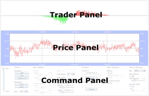
The user interface consists of three parts:
Trader Panel

The Trader Panel visualizes the movement of the single traders. Every trader is represented as a small filled square. Traders possessing a stock (sellers) are red, buyers are green. The window is focused on 1000, the fixed start price of each simulation, and shows the range between 750 and 1250. It is not adjustable.
Price Panel
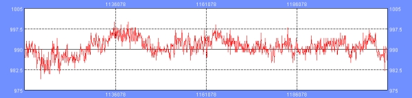
The Price Panel shows the development of the price in time. It commences to display the graph as soon as there is enough data to fill the window with respect to the chosen solution. To make tracking easier every displayed section overlaps a little bit with the last shown one.
Command Panel
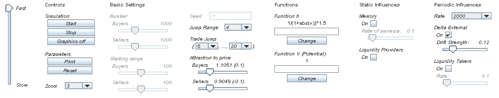
The Command Panel enables one to change the parameters of the simulation. For some parameters this does not always make sense, thus they are sometimes not activatable. As already mentioned we refer to the notation of the paper The Opinion Game. Whenever we do this we emphasize it with the phrase "corresponds to".
The slider on the left side specifies the speed of the simulation. This gives the possibility to track the movements of the traders one by one.
Controls
Start/Pause
-
Starts the simulation (if paused or stopped) or pauses it (if running). In contrast to Stop, Pause preserves the current state of the simulation. When one starts it again the simulator continues from this state.
Stop
-
Stops the simulation completely. This means all development of the simulation is reset and the traders are set to the initial state.
Graphics on/off
-
Switches the Trader and the Price Panel on or off. If one does it while running a simulation, the panels will freeze immediately. When turning on the graphics again the graphical output will correspond to the current state of the simulation.
-
Prints out the current parameters to the standard console.
Reset
-
Resets all parameters to the values mentioned in the footnote on page ten of the paper.
-
Changes the solution of the Price Panel.
1: 10,000 (steps)
2: 50,000 (steps)
3: 100,000 (steps)
4: 500,000 (steps)
If one chooses a solution for which the number of made steps has not been sufficient, yet, the simulator scales the panel such that it is completely filled with the available data.
Basic settings
Most of theses parameters are only changeable if the simulation is stopped.
Number Buyers/Seller
-
Corresponds with N-M (buyers) and M (sellers).
Starting range Buyers/Sellers
-
In the beginning the buyers are uniformly distributed in [1000-x, 999] ∩
Seed
-
The seed determines the sequence of pseudo-random numbers to calculate the outer drift. The same seed always produces the same sequence and therefore also the same outer drift for the same time period. Because this drift drives the behavior of the simulation in a strong way, the choice of the same seed for different runs makes the runs more comparable. The seed must be a nonnegative integer. If the input is negative, it is ignored and the seed is chosen randomly.
Jump Range
-
Corresponds to l.
Remark: ε = 1 (fixed).
Trade Jump
-
Corresponds to r1 and r2.
Attraction to price
-
Corresponds to δB (buyers) and δS (sellers). The logarithm of the current value is stated in the brackets.
Functions
-
The functions correspond to the functions h and V.
The functions are implemented with the JAVA Mathematical Expression parser 2.3.0 (JEP). One can find a detailed description of the possibilities on the homepage. If an input cannot be parsed it is ignored.
Reminder: The start price is 1000. Thus one should be careful about choosing a potential.
Static & Unique Influences
These possibilities have not been described in the paper.
Memory
-
If the memory is switched on, every trader remembers the price of his last trade and do not want to make a worse deal. Thus he will not jump over the last trade-price.
In addition one can introduce a probability of flouting this rule (rate of amnesia).
Liquidity providers
-
Liquidity providers buy/sell stocks for the bid/ask price. Thus, if somebody wants to trade the liquidity providers always have the best offer. They make their profit by the difference between the bid and the ask price.
In the simulation tool this is simulated by setting the trading partner (assuming he is a liquidity provider) always to the bid (if he is the seller) or ask price (if he is the buyer), resp. There is no extra trading jump for him.
Big orders
-
Enables you to put specific big orders into the market. As soon as you click on "Buy" or "Sell", resp., only traders of the concerning group are chosen uniformly for the next n steps, where n is the order size. Then these market participants are forced to trade. Also the step after the trade is not performed as usual. Instead the traders chose the new positions randomly, whereby the current market configuration defines the probability measure. Notice that this only holds for buyers/sellers if you have clicked on "Buy"/"Sell". The trading partners behave as usual. After executing a big order the applet shows the relative price impact below. To keep the numbers reasonable, we assume that the underlying grid size is .01.
Periodic Influences
Rate
-
Corresponds to 1/ω.
Delta external
-
First of all you can switch off the external drift completely. If it is switched on the drift strength corresponds to the mean of the exponential distributed random variables s'i.
Liquidity takers
-
This is another feature which is has not been covered by the paper.
A liquidity provider want to trade a large amount of stocks. If he tried to trade them at once he would influence the market price in a unfavorable way (from his point of view). Thus he splits his orders in smaller pieces and spreads them over a certain time horizon.
In the simulation tool we implemented this behavior by introducing a rate for trading at once, independent of the traders current position. The probability for this event is given by the rate. It is not reasonable to assume one places his orders against the price trends (driven by the external drift). Therefore liquidity takers always move into the direction of the external drift (even if this drift is switched off, it is still calculated inside the program).
- If the function values of the parsed functions are too big, the parser returns NaN (Not a number) and the behavior of the program becomes unpredictable.
If you find other errors, please send a mail to me.
To do
-
There is also a window-version of the program. It has several advantages. It is faster than the applet version and writes the recorded data (price, price-returns, distance between sellers and buyers, ...) into files. Furthermore it is possible to start it automatically by consigning all parameters with the program call or in a configuration file. As soon as this version is documented, it will hopefully be published on this homepage. If you are too interested to wait, send me a mail.
The (almost identical) source codes of both program versions will not be published on this homepage, but if you are doing research in this area it is maybe possible to give the code to you under the conditions that you do not spread the code on your own and only use it for scientific, non-commercial issues.
Back to
Last modified: May 27, 2010,
Alexander Weiß