[Next]:

Phase transitions

[Previous]:

Sharp interface model for eutectic tin/lead

 [Contents] 

 [Index] 

Micro-macro transitions of the atomic chain for various scalings

Collaborator: W. Dreyer (FG 7), M. Herrmann (FG 7), A. Möller (FG 7), J. Sprekels

(FG 1)

Cooperation with: M. Kunik (Otto-von-Guericke Universität Magdeburg), A. Mielke (Universität Stuttgart)

Supported by: DFG: Priority Program ``Analysis, Modellbildung und Simulation von Mehrskalenproblemen'' (Analysis, modelling and simulation of multiscale problems)

Description:

In this project we study the initial value problem for an atomic chain consisting of a large number N of identical atoms. The dynamics of the chain is governed by Newton's equation

$${}\ddot{x}_\alpha(t) {}\Phi^\prime\Big({x}_{\alpha+1}(t)-{x}_{\alpha}(t)\Big)- \Phi^\prime\Big({x}_{\alpha}(t)-{x}_{\alpha-1}(t)\Big).$$ = (1)

Here $x_\alpha(t)$ denotes the position of the atom $\alpha$ at time t. The interaction potential $\Phi$ is assumed to be nonlinear and convex.

Our main goal is to develop and to apply mathematical methods in order to pass to the macroscopic limit that results if the particle number N tends to infinity.

In the last report period we concentrated on the following setting for micro-macro transitions in the atomic chain.

1.

We consider periodic boundary conditions.

2.

In order to study macroscopic wave phenomena we use the hyperbolic scaling, i.e. time t, space x and particle index $\alpha$ will be scaled in the same way

$${}\overline{t}=\varepsilon{t},\quad\overline{x}=\varepsilon{x},\quad \overline{\alpha}=\varepsilon{\alpha},\quad\varepsilon=1/N.$$ (2)

3.

In order to initialize the atomic distancies $r_{\alpha}=x_{\alpha+1}-x_{\alpha}$ we chose two macroscopic functions r₀¹, r₀² and define

$$r_\alpha(0)=\left\{\begin{array} {lcl} r_0^1(\varepsilon{\al... ...{\alpha})&\text{if}&\alpha\text{ is {even}}.\end{array}\right.$$ (3)

A similar procedure with two functions v₀¹ and v₀² determines the initial atomic velocities.

Next we discuss the special structure of the initial data. If the particle number is sufficiently large, there exist locally only two initial distancies r₀¹, r₀² and two initial velocities v₀¹, v₀² in the atomic chain. However, the values may vary on the macroscopic scale.

There are at least two reasons why these initial data are interesting for micro-macro transitions. Firstly, they pose an effective but simple possibility to create an initial temperature field in the chain. Secondly, in the case that r₀¹, r₀² and v₀¹, v₀² are constant, we can rigorously pass to the limit $N\rightarrow\infty$. All interesting thermodynamical quantities are then determined by a single ODE

$${}\frac{d^{\,2}r}{d\,\tau^2}(\tau) {}\Phi^\prime\big(d-r(\tau)\big)-\Phi^\prime\big(d+r(\tau)\big),\quad 2d=r_0^1+r_0^2.$$ = (4)

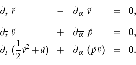
In [1, 2] we start with the assumption that the special structure of our initial data is conserved for macroscopic times $\overline{t}\gt$. We show that if $N\rightarrow\infty$ there results the following system of PDEs

$$\begin{array} {lclcl} \displaystyle{\partial_{\,\overline{t}... ...\overline{\alpha}}\,\;}{(\tilde{p}\,\tilde{v})}&=&0.\end{array}$$ (5)

This system is the well-known Euler system for specific length $\tilde{r}$, velocity $\tilde{v}$, pressure $\tilde{p}$ and specific internal energy $\tilde{u}$. The Euler system is closed by the equation of state

$$\tilde{p}=\tilde{p}\big(\tilde{r},\,\tilde{u}\big),$$ (6)

which can be derived from the ODE (4).

Furthermore, in [1] and [2] we predict the local distribution functions for the atomic velocities and atomic distancies and we derive the Gibbs equation for (5).

Numerical simulations indicate that the above-mentioned assumption leads to an appropriate description of the atomic chain for very large particle numbers. This fact is illustrated by the following figures.

Fig. 1: The initial atomic distancies and velocities

Figure 1 shows the macroscopic initial configuration of a chain with 16000 atoms. The interaction potential is the well-known Toda potential.

Fig. 2: The atomic distancies and velocities for fixed $\overline{t}\gt$

The resulting data for $\overline{t}=0.5$ are depicted in Figure 2. The highly oscillating functions, which are not observable on the macroscopic scale correspond to atomic distancies and velocities. The dark-colored macroscopic curves are the mean values of the microscopic oscillations and represent the specific length $\tilde{r}$and the macroscopic velocity $\tilde{v}$.

The last figure contains four examples of local distribution functions of the atomic distancies. The light-colored and continuous curves have been calculated by means of the macroscopic fields. The dark-colored and dotted curves correspond to the distribution functions according to Newton's equations.

Regarding the numerical solution of the microscopic equation of motion, the Verlet-Stoermer as well as the velocity-Verlet method are used. Both methods are applicable to molecular dynamics, however, the velocity-Verlet method tends to be more suitable to maintain the symplectic structure [3, 6] of the equation.

There follow two examples illustrating some of the numerical studies.

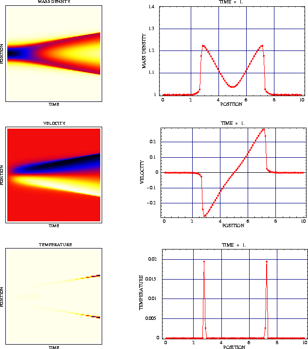
Continuous cold initial data with Gauss-distributed mass densities

(in collaboration with N. Gröwe (Humboldt-Universität zu Berlin), R. Henrion (WIAS: research group ``Nonlinear Optimization and Inverse Problems'')).

For given values $\varrho^{min}$, $\varrho^{max}$ and standard deviation s we define $w := (\varrho^{max} - \varrho^{min}) / f_{G}(0.5, 0.5, s)$ and consider continuous cold initial data of the type $\varrho(x) = \varrho^{min} + w * f_{G}(x/L,0.5,s)$, $v(x) \equiv 0$, $T(x) \equiv 0$. Here f_G denotes the Gaussian distribution density $f_{G}(z,m,s) := \frac{1}{\sqrt{2 \pi} s}\: \exp\left(-\frac{(z-m)^2}{2 s^2} \right)$. For a given atom index $\alpha \in \{0,\ldots,N-1\}$ the initial positions $x_{\alpha}$ of the atoms are iteratively computed by $\alpha := \int_0^{x_{\alpha}} \varrho(x) dx = \int_0^{x_{\alpha}} \varrho^{min}... ...n} * x_{\alpha} + w * L * 0.5 * \mbox{Erf}((x_{\alpha}/L - 0.5) / (\sqrt{2} s))$. Here, an explicit representation of the required chainlength L is available from $N - 1 = \int_0^{x_{N-1}} \varrho(x) dx = \int_0^L \varrho(x) dx = \int_0^L \var... ....5,s) dx = \varrho^{min} * L + 2 * w * L * 0.5 * \mbox{Erf}(1 / (2 \sqrt{2} s))$. For a practial computation of the errorfunction see, e.g., [4]. The data are N = 50001, $\varrho^{min} = 1.0$, $\varrho^{max} = 1.4$, s = 0.06, $\lambda \approx 4716.3$. The numerical results depicted in the pictures below show that temperature may result from cold initial data.

An alternative approach for the generation of initial data for the thermal closure.

In [1] thermal motion of the atomic chain is defined by the following assumptions:

1.

The distributions of the atomic distances and velocities are completely uncorrelated.

2.

The thermal velocities c are distributed by the Gaussian density with mean 0.0 and deviation $\sqrt{T}$

$$f(c) := \frac{1}{\sqrt{2 \pi} \sqrt{T}}\: \exp\left(-\frac{c^2}{2 T}\right).$$

3.

The distances r are distributed by the density function

$$F(r) := \hat{F}(\alpha, \beta, r) := \frac{1}{\int_0^{\inft... ... - \beta \varphi(r))}\: \exp(-\alpha r - \beta \varphi(r)),$$

where $\varphi$ is the potential, $\beta := 1/T$, and $\alpha$ is determined by the mean distance $1/\varrho = \bar{r}(\alpha,\beta) := \int_0^{\infty} r\: \hat{F}(\alpha, \beta, r) dr$.

To prepare the atomic chain in thermal equilibrium, in [1] Section 9.2, the authors start with an equidistant distribution of the distances $r \equiv L/(N-1)$ and a distribution of the thermal velocities according to some auxiliary temperature $T^{\prime}$. Solving the microscopic equation of motion after some iteration the distributions f(v) and F(r) will appear approximately.

To overcome the pre-iterations, the distribution of the velocities may be simulated by a random number generator for the Gaussian distribution as above using the initial temperature T instead of the auxiliary temperature $T^{\prime}$.Since the cumulative distribution function of F is bijective, the distances may be generated by the inverse transform method [5]. For this purpose a sequence of random numbers $\{u_1,\ldots,u_N,\ldots\}$ will be generated which are uniformly distributed on [0,1]. Next the distances are initialized by r_i := G^-1(u_i) where G denotes the distribution function of F. Then the resulting sequence $\{r_1,\ldots,r_N,\ldots\}$ will be distributed according to the density F.

References:

1. W. DREYER, M. KUNIK, Cold, thermal and oscillator closure of the atomic chain, WIAS Preprint no. 489 , 1999.
2. W. DREYER, M. HERRMANN, Towards rigorous micro-macro transitions: The microscopic oscillator motion, WIAS Preprint no. 724 , 2002.
3. W. DREYER, R. GUCKEL, Micro-macro transition by interpolation, averaging, and scaling of particle trajectories, with applications to the atomic spin chain, WIAS Preprint no. 725 , 2002.
4. dcdflibf.uuen: Library for calculating double precision cumulative distribution functions and their inverses, URL: http://lib.stat.cmu.edu/general/Utexas/ .
5. G.S. FISHMANN, Monte Carlo: Concepts, Algorithms, and Applications, Springer Series in Operations Research, Springer, New York [...], 1996.
6. R.D. SKEEL, G. ZHANG, T. SCHLICK, A family of symplectic integrators: Stability, accuracy, and molecular dynamics applications, SIAM J. Sci. Comput., 18 (1997), pp. 203-222.

[Next]:

Phase transitions

[Previous]:

Sharp interface model for eutectic tin/lead

 [Contents] 

 [Index]