Path planning for robots and human

Theoretical insights about the
- attainability of (welding) points,
- choice of robot type,
- placement of robots, workpieces, grippers, etc.
- cycle times,
offline computation of robot controls,
visualization of the whole process (movements of robot and man),
direct coupling of robot control to the simulation software,
generation of programs for the robot control,
processing of the original robot programs.

In the field of path planning for robots, the work is built up on previous joint efforts with the industrial partner and is focused on practice-related extensions for synchronization and modification. Among other things, the preservation of speed limits for the TCP (tool center point) for linear paths has been realized.

The path planning for human models has been implemented in a first attempt analogously to the one of the robot models. We are proceeding on the assumption of a simplified axes model. The overparametrization of the final position and final hand orientation is resolved by independently determining the positions of the trunk and the shoulder.

Inverse kinematics

The position and the orientation of a point in space are given by six coordinates, three for the position vector (v) and three for the local orientation.

The orientation is described by a rotation matrix (R) to be produced by rotations executed one after the other on three independent axes.

A transformation of an oriented point consists of a translation and a rotation. A point can be identified by the transformation of the point of origin ( $v_0=(0,0,0), R_0 = \textrm{Id}$ ).

Thus, the transformations form a (noncommutative) group as far as the execution one after the other is concerned.

Point coordinates and orientation can be given absolutely, i.e. in connection with a world coordinate system, or relatively, i.e. in respect of a local coordinate system.

The transformation in local coordinates corresponds to the multiplication on the left-hand side, the transformation of the global coordinates to the transformation on the right-hand side.

Transformation on the left-hand side

(local coordinate system)

$\begin{eqnarray*} T_r(v,R):\qquad (v_n,R_n) & = & T_r(v,R)(v_a,R_a),\textrm{~with}\ [5pt] v_n & = & v_a + R_a * v \ R_n & = & R_a * R\end{eqnarray*}$

Transformation on the right-hand side

(global coordinate system)

$\begin{eqnarray*} T_l(v,R):\qquad (v_n,R_n) & = & T_l(v,R)(v_a,R_a),\textrm{~with}\ [5pt] v_n & = & v + R * v_a \ R_n & = & R * R_a\end{eqnarray*}$

**Fig. 1:** Simulated ramps in comparison with measured ones
$%% \ProjektEPSbildNocap {0.8\textwidth}{transform.eps}$

The direct kinematics

consist of the calculation of the position and orientation of a point in space by multiplying individual parameter-dependent transformations. In the case of robot kinematics, these parameters are the lengths and the angles of the axes. The lengths of the axes are (in general) fixed. Some angles are determined by the position of the motor in the joints. Thus they are free. In addition, the temporal changes of the parameters being given, the path is calculated in its final point, as a function of time.

The inverse problem

consists of the calculation of the transformation parameters (positions of the axes) from given point coordinates and orientations and the calculation of the angular speed for given paths.

Ramp model

The real robot controls realize the axial movements in so-called ramps, i.e. the velocity profile is, in its idealized form, piecewise linear.

$\begin{displaymath} \omega(t) := \left\{ \begin{array} {ll} b_a t, & t \le t_1\... ...t \le t_2 \ b_a t_1 - b_e(t-t_2), & t_2 < t\end{array} \right.\end{displaymath}$

For a simple movement, consisting of a phase of acceleration to a constant velocity and a phase of deceleration, this results in the form of a trapezoid for the velocity graph.

For each axis, the lengths of the phases of acceleration and of the interval with constant angular speed are computed for given angle differences and time slices.

Since all axes are supposed to conclude their movement synchronously, we first compute, for each axis, the minimal time to reach the new position. Then we determine the time slice for the whole movement as the maximum of these times.

The axis requiring the longest time for its movement is called the leading axis. This one works with maximum velocity and determines the time slice for all other axes.

The calculation of the ramp profiles for given time slices entails piecewise quadratic equations.

A path leading through several points is constructed from individual ramp profiles.

In a PTP (point to point) run with zero velocity in the point to be reached, the ramps are clearly defined and directly to be determined.

In a ``sliding over'' run, the point is passed by without stopping. This is realized by subsidiary points in which the velocity has not to be zero.

Thus we get an optimization problem with free velocities in the individual points of the path.

The approximate solution

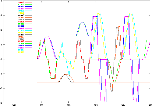
of the optimization problem for paths through several points is obtained by a direct method, starting out from maximal transit velocities and taking only the accessibility of the next point into consideration. In this process, it is possible that an already calculated ramp has to be corrected in case that the transit velocities have been too high to reach the arrival point exactly.

The figure shows a relatively good agreement of the ramp model with the real robot control.

$\begin{figure} \ProjektEPSbildNocap {\textwidth}{rampenr.ps.gz} \end{figure}$

**Fig. 2:** Axes in the human model
$%% \ProjektEPSbildNocap {0.7\textwidth}{worker-axis.eps.gz}$

Human model

Kinematics for the ,,worker``

Position of the local coordinate system to the world coordinate system fixes the pelvis area.
The upper part of the body is fixed with reference to the pelvis (i.e. in the local coordinate system),
the arms relatively to the shoulders (determined by the upper part of the body), and
the legs relatively to the hip (determined by the pelvis).

Inverse problem

given:: position of hands and feet in world coordinates.
searched:: angles for all joints

Reduced inverse problem

given:: position of pelvis, hands, and feet
searched:: angle for the rotation of the upper part of the body and of the joints of arms and legs

Path calculation for motion sequences

Example: walking straight ahead

Decomposition of the motion sequence into three sub-sequences: ``foot up'', ``foot forward'', ``foot down'',
positioning of the trunk in the intermediate points,
positioning of the legs, one foot fixed,
positioning of the hands for balancing movements of the arms,
independent path calculation for the individual kinematics,
on-line correction of the fixed foot on the surface of the path (by use of SQP methods).

References:

H.G. BOCK, J.P. SCHLÖDER, M.C. STEINBACH, H. WÖRN, V.H. SCHULZ, R.W. LONGMAN, Schnelle Roboter am Fließband: Mathematische Bahnoptimierung in der Praxis, in: Mathematik -- Schlüsseltechnologie für die Zukunft, K.-H. Hoffmann, W. Jäger, Th. Lohmann, H. Schunck, eds., Springer, Berlin, Heidelberg, 1997, pp. 539-550.
M.C. STEINBACH, H.G. BOCK, G.V. KOSTIN, R.W. LONGMAN, Mathematical optimization in robotics: Towards automated high speed motion planning, Surveys Math. Indust., 7 (1998), pp. 303-340.

[Next]:

Parameter estimation in multiphase flow

[Up]:

Project descriptions

[Previous]:

Optimization problems with random and nonsmooth

[Contents]

[Index]

LaTeX typesetting by I. Bremer
9/9/2002