xxxxxxxxxx
 
begin 
    ENV["LANG"]="C"
    using Pkg
    Pkg.activate(mktempdir())
    using Revise
    Pkg.add("Revise")
    Pkg.add(["PyPlot","PlutoUI","ExtendableGrids","GridVisualize", "VoronoiFVM"])
    using PlutoUI,PyPlot,ExtendableGrids,VoronoiFVM,GridVisualize
    PyPlot.svg(true)
end;

13.2 s

Finite volumes: transient problems

4.6 μs

Construction of control volumes

Start with a triangulation of a polygonal domain (intervals in 1D,triangles in 2D, tetrahedra in 3D).
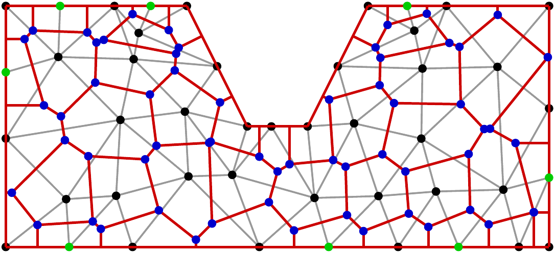
Join triangle circumcenters by lines $\to$ create Voronoi cells which can serve as control volumes, akin to representative elementary volumes (REV) used to derive conservation laws.

Black + green: triangle nodes
Gray: triangle edges
Blue: triangle circumcenters
Red: Boundaries of Voronoi cells

32.6 ms

Condition on triangulation

There is a 1:1 incidence between triangulation nodes and Voronoi cells. Moreover, the angle between the interface between two Voronoi cells and the edge between their corresponding nodes is $\frac{π}{2}$ .
Requires (in 2D) that sums of angles opposite to triangle edges are less than $π$ and that angles opposite to boudary edges are less than $\frac{π}{2}$ .
"boundary conforming Delaunay property". It has different equivalent definitions and analogues in 3D.
Construction:
- "by hand" (or script) from tensor product meshes
- Mesh generators: Triangle, TetGen
- Julia packages: Triangulate.jl, TetGen.jl; SimplexGridFactory.jl

11.7 μs

The discretization approach

Use Voronoi cells as REVs aka control volumes aka finite volume cells.

16.5 μs

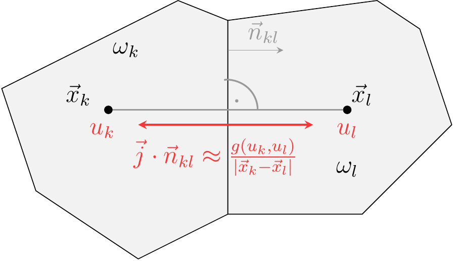
Given a continuity equation $\nabla \cdot \vec{j} = 0$ in a domain $Ω$ , integrate this over a contol volume $ω_{k}$ with associated node ${\vec{x}}_{k}$ and apply Gauss theorem:

$\begin{aligned} 0 & = \int_{ω_{k}} \nabla \cdot \vec{j} d ω = \int_{\partial ω_{k}} \vec{j} \cdot \vec{n} d s \\ = \sum_{l \in N_{k}} \int_{ω_{k} \cap ω_{l}} \vec{j} \cdot \vec{n} d s + \int_{\partial ω_{k} \cap \partial Ω} \vec{j} \cdot \vec{n} d s \\ \approx \sum_{l \in N_{k}} \frac{σ_{k l}}{h_{k l}} g (u_{k}, u_{l}) + γ_{k} b (u_{k}) \end{aligned}$

Here, $N_{k}$ is the set of neighbor control volumes, $σ_{k l} = | ω_{k} \cap ω_{l} |$ , $h_{k l} = | {\vec{x}}_{k} - {\vec{x}}_{l} |$ , $γ_{k} = | \partial ω_{k} \cap \partial Ω |$ , where $| \cdot |$ denotes the measure (length resp. area) of a geometrical entity.

6.5 μs

Flux functions

For instance, for the diffusion flux $\vec{j} = - D \vec{\nabla} u$ , we use $g (u_{k}, u_{l}) = D (u_{k} - u_{l})$ .

For a convective diffusion flux $\vec{j} = - D \vec{\nabla} u + u \vec{v}$ , one can chose the upwind flux

$\begin{aligned} g (u_{k}, u_{l}) = D (u_{k} - u_{l}) + v_{k l} {\begin{cases} u_{k}, & v_{k l} > 0 \\ u_{l}, & v_{k l} \leq 0, \end{cases} \end{aligned}$

where $v_{k l} = \frac{h_{k l}}{σ_{k l}} \int_{ω_{k} \cap ω_{l}} \vec{v} \cdot {\vec{n}}_{k l} d s$ Fluxes also can depend nonlinearily on $u$ .

5.6 μs

Software API and implementation

$\partial_{t} s (u) + \nabla \cdot \vec{j} (u) + r (u) = f$

The entities describing the discrete system can be subdivided into two categories:

geometrical data: $| ω_{k} |, γ_{k}, σ_{k l}, h_{k l}$ together with the connectivity information of the triangles
physical data: the number $m$ and the functions $s, g, r, f$ describing the particular problem, where $g$ is a flux function approximating $\vec{j}$ .

This structure allows to describe the problem to be solved by data derived from the discretization grid and by the functions describing the physics, giving rise to a software API.

The solution of the nonlinear systems of equations can be performed by Newton's method combined with various direct and iterative linear solvers.

The generic programming capabilities of Julia allow for an implementation of the method which results in an API which consists in the implementation of functions $s, g, r, f$ without the need to write code for their derivatives.

7.8 μs

Examples

General settings

Initial value problem with homgeneous Neumann boundary conditions

$Ω = (0, 1)^{d}, d = 1, 2$

$T = [0, t_{e n d}]$

4.2 μs

fpeak (generic function with 2 methods)

xxxxxxxxxx
 
# Define function for initial value $u_0$ with two methods - for 1D and 2D problems
begin
    fpeak(x)=exp(-100*(x-0.25)^2)
    fpeak(x,y)=exp(-100*((x-0.25)^2+(y-0.25)^2))
end

23.7 μs

create_grid (generic function with 1 method)

xxxxxxxxxx
 
# Create discretization grid in 1D or 2D with approximately n nodes
function create_grid(n,dim)
    nx=n
    if dim==2
        nx=ceil(sqrt(n))
    end
    X=collect(0:1.0/nx:1)
    if dim==1
      grid=simplexgrid(X)
    else
      grid=simplexgrid(X,X)
    end
end

21.5 μs

Diffusion problem

$\partial_{t} u - \nabla \cdot D \nabla u = 0 in Ω$

$D \nabla u \cdot \vec{n} = 0 on \partial Ω$

$u |_{t = 0} = u_{0}$

2.9 μs

diffusion (generic function with 1 method)

xxxxxxxxxx
 
function diffusion(;n=100,dim=1,tstep=1.0e-4,tend=1, D=1.0, dtgrowth=1.1)
    grid=create_grid(n,dim)
    
    ## Diffusion flux between neigboring control volumes
    function flux!(f,u,edge)
        uk=viewK(edge,u)  
        ul=viewL(edge,u)
        f[1]=D*(uk[1]-ul[1])
    end
​
    ## Storage term (under time derivative)
    function storage!(f,u,node)
        f[1]=u[1]
    end
​
    ## Create a physics structure
    physics=VoronoiFVM.Physics(
        flux=flux!,
        storage=storage!)
    
    sys=VoronoiFVM.DenseSystem(grid,physics)
    enable_species!(sys,1,[1])
    
    ## Create a solution array
    inival=unknowns(sys)
​
    ## Broadcast the initial value
    inival[1,:].=map(fpeak,grid)
​
    control=VoronoiFVM.NewtonControl()
    control.Δt_min=0.01*tstep
    control.Δt=tstep
    control.Δt_max=0.1*tend
    control.Δu_opt=0.1
    control.Δt_grow=dtgrowth
    
    tsol=solve(inival,sys,[0,tend];control=control)
    return grid,tsol
end 

87.4 μs

xxxxxxxxxx
 
grid_diffusion,tsol_diffusion=diffusion(dim=1,n=100);

10.2 s

TransientSolution{Float64, 3, Vector{Matrix{Float64}}, Vector{Float64}}

xxxxxxxxxx
 
typeof(tsol_diffusion)

62.0 ns

Documentation for NewtonControl
Documentation for transient solve
Documentation for TransientSolution

7.9 μs

Time step number:1

25.8 ms

820 ms

790 ms

Reaction-diffusion problem

Diffusion + physical process which "eats" species

$\partial_{t} u - \nabla \cdot D \nabla u + R u = 0 in Ω$

$D \nabla u \cdot \vec{n} = 0 on \partial Ω$

$u |_{t = 0} = u_{0}$

8.0 μs

reaction_diffusion (generic function with 1 method)

xxxxxxxxxx
 
​
function reaction_diffusion(;
        n=1000,
        dim=1,
        tstep=1.0e-4,
        tend=1, 
        D=1.0, 
        R=10.0, 
        dtgrowth=1.1)
​
    grid=create_grid(n,dim)
    ## Diffusion flux between neigboring control volumes
    function flux!(f,u,edge)
        uk=viewK(edge,u)  
        ul=viewL(edge,u)
        f[1]=D*(uk[1]-ul[1])
    end
​
    ## Storage term (under time derivative)
    function storage!(f,u,node)
        f[1]=u[1]
    end
​
    ## Reaction term
    function reaction!(f,u,node)
        f[1]=R*u[1]
    end
​
  
    ## Create a physics structure
    physics=VoronoiFVM.Physics(
        flux=flux!,
        reaction=reaction!,
        storage=storage!)
    
    sys=VoronoiFVM.DenseSystem(grid,physics)
    enable_species!(sys,1,[1])
    ## Create a solution array
    inival=unknowns(sys)
    
    ## Broadcast the initial value
    inival[1,:].=map(fpeak,grid)
​
    
    
    control=VoronoiFVM.NewtonControl()
    control.Δt_min=0.01*tstep
    control.Δt=tstep
    control.Δt_max=0.1*tend
    control.Δu_opt=0.1
    control.Δt_grow=dtgrowth
    
    tsol=solve(inival,sys,[0,tend];control=control)
    return grid,tsol
end

118 μs

xxxxxxxxxx
 
grid_rd,tsol_rd=reaction_diffusion(dim=1,n=100,R=10);

1.3 s

Time step number:1

xxxxxxxxxx
 
md"""
Time step number:$(@bind t_reaction_diffusion Slider(1:length(tsol_rd),default=1,show_value=true))
"""

46.9 μs

106 ms

4.3 ms

Convection-Diffusion problem

$\partial_{t} u - \nabla \cdot (D \nabla u - u \vec{v}) = 0 in Ω$

$(D \nabla u - u \vec{v}) \cdot \vec{n} = 0 on \partial Ω$

$u |_{t = 0} = u_{0}$

4.7 μs

convection_diffusion (generic function with 1 method)

xxxxxxxxxx
 
function convection_diffusion(;
        n=20,
        dim=1,
        tstep=1.0e-4, 
        tend=1, 
        D=0.01, 
        vx=10.0,
        vy=10.0,
        dtgrowth=1.1, 
        scheme="expfit")
   grid=create_grid(n,dim)
   # copy vx, vy into vector
   if dim==1
        V=[vx]
   else
        V=[vx,vy]
   end
   # Bernoulli function
    
    
    B(x)=x/(exp(x)-1)
 
    function flux_expfit!(f,u,edge)
        uk=viewK(edge,u)  
        ul=viewL(edge,u)
        vh=project(edge,V)  # Calculate projection v * (x_L-x_K)
        f[1]=D*(B(-vh/D)*uk[1]- B(vh/D)*ul[1])
    end
    
    function flux_centered!(f,u,edge)
        uk=viewK(edge,u)  
        ul=viewL(edge,u)
        vh=project(edge,V)
        f[1]=D*(uk[1]-ul[1])+ vh*0.5*(uk[1]+ul[1])
    end
    
    function flux_upwind!(f,u,edge)
        uk=viewK(edge,u)  
        ul=viewL(edge,u)
        vh=project(edge,V)
        f[1]=D*(uk[1]-ul[1])+ ( vh>0.0 ? vh*uk[1] : vh*ul[1] )
    end
    
    flux! =flux_upwind!
    if scheme=="expfit"
        flux! =flux_expfit!
    elseif scheme=="centered"
        flux! =flux_centered!
    end
    
    
    ## Storage term (under time derivative)
    function storage!(f,u,node)
        f[1]=u[1]
    end
​
    ## Create a physics structure
    physics=VoronoiFVM.Physics(
        flux=flux!,
        storage=storage!)
    
    sys=VoronoiFVM.DenseSystem(grid,physics)
    enable_species!(sys,1,[1])
    ## Assume homogeneous Neumann boundary conditions, so do nothig
    
    ## Create a solution array
    inival=unknowns(sys)
    
    ## Broadcast the initial value
    inival[1,:].=map(fpeak,grid)
​
    
    control=VoronoiFVM.NewtonControl()
    control.Δt_min=0.01*tstep
    control.Δt=tstep
    control.Δt_max=0.1*tend
    control.Δu_opt=0.1
    control.Δt_grow=dtgrowth
    
    tsol=solve(inival,sys,[0,tend];control=control)
    return grid,tsol
end 

161 μs

scheme:

116 ms

xxxxxxxxxx
 
grid_conv,tsol_conv=convection_diffusion(n=100,
    dim=1,
    scheme=scheme[1],
    vx=10,vy=10);

2.1 s

Time step number:1

45.3 μs

37.8 ms

4.2 ms

Brusselator system

Two species interacting via a reaction:

$\begin{aligned} \partial_{t} u_{1} - \nabla \cdot (D_{1} \nabla u_{1}) & + (B + 1) u_{1} - A - u_{1}^{2} u_{2} = 0 \\ \partial_{t} u_{2} - \nabla \cdot (D_{2} \nabla u_{2}) & + u_{1}^{2} u_{2} - B u_{1} = 0 \end{aligned}$

4.5 μs

brusselator (generic function with 1 method)

xxxxxxxxxx
 
function brusselator(;n=100,dim=1,A=4.0,B=6.0,D1=0.01,D2=0.1,perturbation=0.1,
    tstep=0.01, tend=150,dtgrowth=1.05)
​
    grid=create_grid(n,dim)
    function storage!(f,u,node)
        f.=u
    end
​
    
function bruss_diffusion!(f,_u,edge)
        u=unknowns(edge,_u)
    f[1]=D1*(u[1,1]-u[1,2])
    f[2]=D2*(u[2,1]-u[2,2])
end
# Reaction:
function bruss_reaction!(f,u,node)
    f[1]= (B+1.0)*u[1]-A-u[1]^2*u[2]
    f[2]= u[1]^2*u[2]-B*u[1]
end
# Create system
bruss_physics=VoronoiFVM.Physics(flux=bruss_diffusion!,storage=storage!,
                                 num_species=2,reaction=bruss_reaction!)
brusselator_system=VoronoiFVM.DenseSystem(grid,bruss_physics)
enable_species!(brusselator_system,1,[1])
enable_species!(brusselator_system,2,[1])
​
    inival=unknowns(brusselator_system)
for i=1:num_nodes(grid)
    inival[1,i]=1.0+perturbation*randn()
    inival[2,i]=1.0+perturbation*randn()
end
​
    
    control=VoronoiFVM.NewtonControl()
    control.Δt_min=0.0001*tstep
    control.Δt=tstep
    control.Δt_max=0.1*tend
    control.Δu_opt=0.1
    control.Δt_grow=dtgrowth
    
    tsol=solve(inival,brusselator_system,[0,tend];control=control)
    return grid,tsol
end
​

128 μs

xxxxxxxxxx
 
grid_bruss,tsol_bruss=brusselator(n=500,dim=1);

4.3 s

Time step number:365

45.7 μs

77.5 ms

50.8 ms

69.0 ns

      Status `/tmp/jl_1ZzYoO/Project.toml`
  [cfc395e8] ExtendableGrids v0.7.4
  [5eed8a63] GridVisualize v0.1.5
  [7f904dfe] PlutoUI v0.7.4
  [d330b81b] PyPlot v2.9.0
  [295af30f] Revise v3.1.14
  [82b139dc] VoronoiFVM v0.10.9

663 ms