Mesh generation

• Regard boundary value problems for PDEs in a finite domain $\mathrm{\Omega }\subset {\mathbb{R}}^d$

• Solution spaces for PDEs are infinite dimensional $\Rightarrow$ develop finite dimensional approximations

• One way of defining such approximations is based on the subdivision of $\mathrm{\Omega }$ into a finite number of elementary closed subsets $T_1\dots T_M$, called mesh or grid

• Elementary shapes:

  • triangles or quadrilaterals ($d=2$)

  • tetrahedra or cuboids ($d=3$)

  • more general cases possible

• During this course:

  • Assume the domain is polygonal, its boundary $\partial \mathrm{\Omega }$ is the union of a finite number of subsets of hyperplanes in ${\mathbb{R}}^n$ (line segments for $d=2$, planar polygons for $d=3$)

  • Focus on simplexes (triangles, tetrahedra)

    • Geometrically most flexible

    • Starting point for more general methods

  • Focus on $d=2$

Admissible grids

Definiton: A grid $\{T_1\dots T_M\}$ of $\mathrm{\Omega }$ is admissible if

• $\mathrm{\Omega }$ is the union of the elementary cells: $\overline{\mathrm{\Omega }}={\cup }_{m=1}^M{T}_m$

• If $T_m\cap T_n$ consists of exactly one point, then this point is a common vertex of $T_m$ and $T_n$.

• If for $m\ne n$, $T_m\cap T_n$ consists of more than one point, then $T_m\cap T_n$ is a common edge (or a common facet for $d=3$) of $T_m$ and $T_n$.

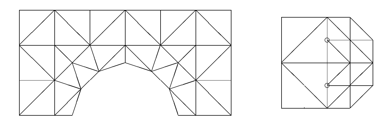
Image (Source: Braess): Left - admissible mesh, right - mesh with "hanging" nodes

• There are generalizations of finite element and finite volume methods which can work with hanging nodes, however we will not go into these details in the course.

Voronoi diagram

After G. F. Voronoi, 1868-1908

Definition: Let $\mathbf{p},\mathbf{q}\in {\mathbb{R}}^d$. The set of points $H_{\mathbf{p}\mathbf{q}}=\{\mathbf{x}\in {\mathbb{R}}^d:||\mathbf{x}-\mathbf{p}||\le ||\mathbf{x}-\mathbf{q}||\}$ is the half space of points $\mathbf{x}$ closer to $\mathbf{p}$ than to $\mathbf{q}$.

Definition: Given a finite set of points $S\subset {\mathbb{R}}^d$, the Voronoi region (Voronoi cell) of a point $\mathbf{p}\in S$ is the set of points $\mathbf{x}$ closer to $\mathbf{p}$ than to any other point $\mathbf{q}\in S$: $V_{\mathbf{p}}=\{\mathbf{x}\in {\mathbb{R}}^d:||\mathbf{x}-\mathbf{p}||\le ||\mathbf{x}-\mathbf{q}||\mathrm{\forall }\mathbf{q}\in S\}$

The Voronoi diagram of $S$ is the collection of the Voronoi regions of the points of $S$.

• The Voronoi diagram subdivides the whole space into ``nearest neigbor'' regions

• Being intersections of half planes, the Voronoi regions are convex sets

Delaunay triangulation

After B.N. Delaunay (Delone), 1890-1980

• Given a finite set of points $S\subset {\mathbb{R}}^d$

• Assume that the points of $S$ are in general position, i.e. no $d+2$ points of $S$ are on one sphere (in 2D: no 4 points on one circle)

  • Connect each pair of points whose Voronoi regions share a common edge with a line $\Rightarrow$ Delaunay triangulation of the convex hull of $S$

Another Interactive example via GEOGRAM. This smoothes the point set after insertion, but you get a good impression about the Duality between Voronoi and Delaunay.

• The circumsphere (circumcircle in 2D) of a $d$-dimensional simplex is the unique sphere containing all vertices of the simplex

• The circumball (circumdisc in 2D) of a simplex is the unique (open) ball which has the circumsphere of the simplex as boundary

Definition: A triangulation of the convex hull of a point set $S$ has the Delaunay property if each simplex (triangle) of the triangulation is Delaunay, i.e. its circumsphere (circumcircle) is empty wrt. $S$, i.e. it does not contain any points of $S$.

• The Delaunay triangulation of a point set $S$, where all points are in general position is unique and has the Delaunay property

• Otherwise there is an ambiguity - if e.g. 4 points are one circle, there are two ways to connect them resulting in Delaunay triangles

Edge flips and locally Delaunay edges (2D only)

• For any two triangles $\mathbf{a}\mathbf{b}\mathbf{c}$ and $\mathbf{a}\mathbf{d}\mathbf{b}$ sharing a common edge $\mathbf{a}\mathbf{b}$, there is the edge flip operation which reconnects the points in such a way that two new triangles emerge: $\mathbf{a}\mathbf{d}\mathbf{c}$ and $\mathbf{c}\mathbf{d}\mathbf{b}$.

• An edge of a triangulation is locally Delaunay if it either belongs to exactly one triangle, or if it belongs to two triangles, and their respective circumdisks do not contain the points opposite wrt. the edge

• If an edge is locally Delaunay and belongs to two triangles, the sum of the angles opposite to this edge is less or equal to $\pi$.

• If all edges of a triangulation of the convex hull of $S$ are locally Delaunay, then the triangulation is the Delaunay triangulation

• If an edge is not locally Delaunay and belongs to two triangles, the edge emerging from the corresponding edge flip will be locally Delaunay

Flip edge to make the triangles Delaunay:

Lawson's Edge flip algorithm for constructing a Delaunay triangulation

This is one of the most elementary mesh generation algorithms

• Input: A stack $L$ of edges of a given triangulation of a set $S$ of $n$ points

• While $L\ne \mathrm{\varnothing }$

  • pop an edge $\mathbf{a}\mathbf{b}$ from $L$

  • If $\mathbf{a}\mathbf{b}$ is not locally Delaunay

    • Flip $\mathbf{a}\mathbf{b}$ to $\mathbf{c}\mathbf{d}$

    • Push edges $\mathbf{a}\mathbf{c},\mathbf{c}\mathbf{b},\mathbf{d}\mathbf{b},\mathbf{d}\mathbf{a}$ onto $L$

This algorithm is known to terminate after $O(n^2)$ operations. After termination, all edges will be locally Delaunay, so the output is the Delaunay triangulation of $S$.

• Among all triangulations of a finite point set $S$, the Delaunay triangulation maximises the minimum angle of all triangles2

• The set of all possible triangulations of $S$ is connected via the flip graph. Each edge of this graph corresponds to one particular flip operation

Randomized incremental flip algorithm (2D only)

• Create Delaunay triangulation of point set $S$ by inserting points one after another, and creating the Delaunay triangulation of the emerging subset of $S$ using the flip algorithm

• Estimated complexity: $O(n\log n)$

• In 3D, there is no simple flip algorithm, generalizations are active research subject

Open source codes implementing mesh generation

• CGAL: The Computational Geometry Algorithms Library

• ND: qhull mostly for pointsets

• 2D: Triangle by J.R.Shewchuk (UC Berkeley)

• 3D: TetGen by H. Si (WIAS Berlin)

• 3D: NetGen by J. Schöberl and coworkers

Triangle

During this course, we will focus on Triangle. It can be compiled to a standalone executable reading and writing files or to a library which can be called from applications.

In Julia it is accessible via the package Triangulate.jl.

The following examples have been taken from that package and slightly modified for Pluto.

General use

• Triangle communicates via a data structure TriangulateIO which contains possible input and output information

• It processes an input structure and returns on output the triangulation, and possibly, the Voronoi diagram.

• It is controlled via a string containing switches

• The switch '-Q' makes Triangle quiet

Delaunay triangulation of the convex hull of a pointset

Create a set of random points in the plane and calculate the Delaunay triangulation of this set of points. It is a triangulation where for each triangle, the interior of its circumcircle does not contain any points of the trianglation.

The Delaunay triangulation of a set of points in general position (no 4 of them on a circle) is unique. At the same time, it is a triangulation of the convex hull of these points.

Given an input list of points, without any further flags, Triangle creates just this triangulation (the "Q" flag suppresses the text output of Triangle). For this and the next examples, the input list of points is created randomly, but on a raster, preventing the appearance of too close points.

Delaunay triangulation of point set with boundary

Same as the previous example, but in addition specify the "c" flag In this case, Triangle outputs an additional list of segments describing the boundary of the convex hull. In fact this is a constrained Delaunay triangulation (CDT) where the boundary segments are the constraining edges which must appear in the output.

Delaunay triangulation of point set with Voronoi diagram

Same as the previous example, but instead of "c" specify the "v" flag In this case, Triangle outputs information about the Voronoi diagram of the point set which is a structure dual to the Delaunay triangulation.

The Voronoi cell around a point $p$ a point set $S$ is defined as the set of points $x$ such that $|x-p|<|x-q|$ for all $q\in S$ such that $p\ne q$.

The Voronoi cells of boundary points of the convex hull are of infinite size. The corners of the Voronoi cells are the circumcenters of the triangles. They can be far outside of the triangulated domain.

Boundary conforming Delaunay triangulation of point set

Specify "c" flag for convex hull segments, "v" flag for Voronoi and "D" flag for creating a boundary conforming Delaunay triangulation of the point set. In this case additional points are created which split the boundary segments and ensure that all triangle circumcenters lie within the convex hull. Due to random input, there may be situations where Triangle fails with this task, so we check for the corresponding exception.

Constrained Delaunay triangulation (CDT) of a domain given by a segment list specifying its boundary.

Constrained Delaunay triangulation (CDT) of a point set with additional constraints given a priori. This is obtained when specifying the "p" flag and an additional list of segments each described by two points which should become edges of the triangulation. Note that the resulting triangulation is not Delaunay in the sense given above.

Constrained Delaunay triangulation (CDT) of a domain given by a segment list specifying its boundary together with a maximum area constraint.

This constraint is specfied as a floating point number given after the -a flag. Be careful to not give it in the exponential format as Triangle would be unable to analyse it. Therefore it is dangerous to give a number in the string interpolation and it is better to convert it to a string before using @sprintf. Specifying only the maximum area constraint does not prevent very thin triangles from occuring at the boundary.

Boundary conforming Delaunay triangulation (BCDT) of a domain given by a segment list specifying its boundary

In addition to the area constraint specify the -D flag in order to keep the triangle circumcenters within the domain.

Triangulation of a domain with refinement callback

A maximum area constraint is specified in the unsuitable callback which is activated via the "u" flag if it has been passed before calling triangulate. In addition, the "q" flag allows to specify a minimum angle constraint preventing skinny triangles.

Triangulation of a heterogeneous domain

The segment list specifies its boundary and the inner boundary between subdomains. An additional region list is specified which provides "region points" in regionlist[1,:] and regionlist[2,:]. These kind of mark the subdomains. regionlist[3,:] contains an attribute which labels the subdomains. regionlist[4,:] contains a maximum area value. size(regionlist,2) is the number of regions.

With the "A" flag, the subdomain labels are spread to all triangles in the corresponding subdomains, becoming available in triangleattributelist[1,:]. With the "a" flag, the area constraints are applied in the corresponding subdomains.