Sparse matrices

In the previous lectures we found examples of matrices from partial differential equations which have only 3 of 5 nonzero diagonals. For 3D computations this would be 7 diagonals. One can make use of this diagonal structure, e.g. when coding the progonka method.

Matrices from unstructured meshes for finite element or finite volume methods have a more irregular pattern, but as a rule only a few entries per row compared to the number of unknowns. In this case storing the diagonals becomes unfeasible.

Definition: We call a matrix sparse if regardless of the number of unknowns $N$, the number of non-zero entries per row and per column remains limited by a constant $n_s$

• If we find a scheme which allows to store only the non-zero matrix entries, we would need not more than $N{n}_s=O(N)$ storage locations instead of $N^2$

• The same would be true for the matrix-vector multiplication if we program it in such a way that we use every nonzero element just once: matrix-vector multiplication would use $O(N)$ instead of $O(N^2)$ operations

• What is a good storage format for sparse matrices?

• Is there a way to implement Gaussian elimination for general sparse matrices which allows for linear system solution with $O(N)$ operation ?

• Is there a way to implement Gaussian elimination \emph{with pivoting} for general sparse matrices which allows for linear system solution with $O(N)$ operations?

• Is there any algorithm for sparse linear system solution with $O(N)$ operations?

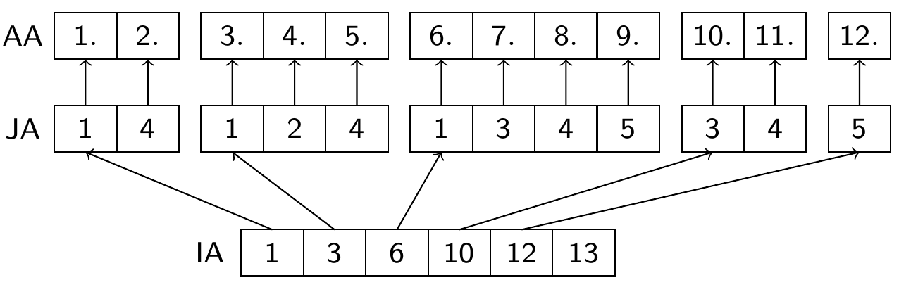
Triplet storage format

• Store all nonzero elements along with their row and column indices

• One real, two integer arrays, length = nnz= number of nonzero elements

(Y.Saad, Iterative Methods, p.92)

• Also known as Coordinate (COO) format

• This format often is used as an intermediate format for matrix construction

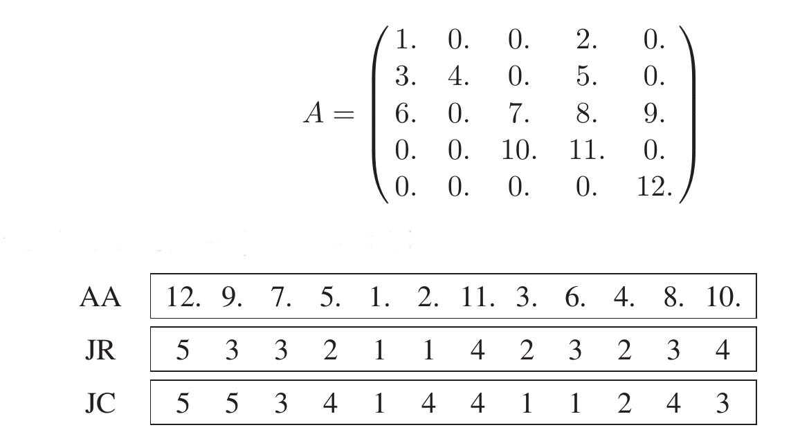
Compressed Sparse Row (CSR) format

(aka Compressed Sparse Row (CSR) or IA-JA etc.)

• float array AA, length nnz, containing all nonzero elements row by row

• integer array JA, length nnz, containing the column indices of the elements of AA

• integer array IA, length N+1, containing the start indizes of each row in the arrays IA and JA and IA[N+1]=nnz+1

$$A=\left(\begin{array}{ccccc}1.& 0.& 0.& 2.& 0.\\ 3.& 4.& 0.& 5.& 0.\\ 6.& 0.& 7.& 8.& 9.\\ 0.& 0.& 10.& 11.& 0.\\ 0.& 0.& 0.& 0.& 12.\end{array}\right)$$

• Used in many sparse matrix solver packages

Compressed Sparse Column (CSC) format

• Uses similar principle but stores the matrix column-wise.

• Used in Julia

Sparse matrices in Julia

Create sparse matrix from a full matrix

Create a random sparse matrix

Random sparse matrix with probability p=0.1 that $A_{ij}$ is nonzero:

Create a sparse matrix from given data

• There are several possibilities to create a sparse matrix for given data

• As an example, we create a tridiagonal matrix.

• Special case: use the Julia tridiagonal matrix constructor

• Create an empty Julia sparse matrix and fill it incrementally

• Use the coordinate format as intermediate storage, and construct sparse matrix from there. This is the recommended way.

• Use the ExtendableSparse.jl package which implicitely uses the so-called linked list format for intermediate storage of new entries. Note the flush!() method which needs to be called in order to transfer them to the Julia sparse matrix structure.

Benchmark summary:

• The incremental creation of a SparseMartrixCSC from an initial state with non nonzero entries is slow because of the data shifts and reallocations necessary during the construction

• The COO intermediate format is sufficiently fast, but inconvenient

• The ExtendableSparse package provides has similar peformance and is easy to use.

Sparse direct solvers

• Sparse direct solvers implement LU factorization with different pivoting strategies. Some examples:

  • UMFPACK: e.g. used in Julia

  • Pardiso (omp + MPI parallel)

  • SuperLU (omp parallel)

  • MUMPS (MPI parallel)

  • Pastix

• Quite efficient for 1D/2D problems - we will discuss this more deeply

• Essentially they implement the LU factorization algorithm

• They suffer from fill-in, especially for 3D problems:

Let $A=LU$ be an LU-Factorization. Then, as a rule, $nnz(L+U)>>nnz(A)$.

• increased memory usage to store L,U

• high operation count

Solution steps with sparse direct solvers

1. Pre-ordering

• Decrease amount of non-zero elements generated by fill-in by re-ordering of the matrix

• Several, graph theory based heuristic algorithms exist

2. Symbolic factorization

• If pivoting is ignored, the indices of the non-zero elements are calculated and stored

• Most expensive step wrt. computation time

3. Numerical factorization

• Calculation of the numerical values of the nonzero entries

• Moderately expensive, once the symbolic factors are available

4. Upper/lower triangular system solution

• Fairly quick in comparison to the other steps

• Separation of steps 2 and 3 allows to save computational costs for problems where the sparsity structure remains unchanged, e.g. time dependent problems on fixed computational grids

• With pivoting, steps 2 and 3 have to be performed together, and pivoting can increase fill-in

• Instead of pivoting, iterative refinement may be used in order to maintain accuracy of the solution

Influence of reordering

• Sparsity patterns for original matrix with three different orderings of unknowns

  • number of nonzero elements (of course) independent of ordering:

  

  (mathworks.com)

• Sparsity patterns for corresponding LU factorizations

  • number of nonzero elements depend original ordering!

  

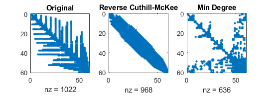
  (mathworks.com)

Sparse direct solvers: Complexity estimate

• Complexity estimates depend on storage scheme, reordering etc.

• Sparse matrix - vector multiplication has complexity $O(N)$

• Some estimates can be given from graph theory for discretizations of heat equation with $N=n^d$ unknowns on close to cubic grids in space dimension $d$

• sparse LU factorization:

$$\begin{array}{ccc}d& work& storage\\ 1& O(N)|O(n)& O(N)|O(n)\\ 2& O(N^{\frac{3}{2}})|O(n^3)& O(N\log N)|O(n^2\log n)\\ 3& O(N^2)|O(n^6)& O(N^{\frac{4}{3}})|O(n^4)\end{array}$$

• triangular solve: work dominated by storage complexity

$$\begin{array}{cc}d& work\\ 1& O(N)|O(n)\\ 2& O(N\log N)|O(n^2\log n)\\ 3& O(N^{\frac{4}{3}})|O(n^4)\end{array}$$

(Source: J. Poulson, PhD thesis)

Practical use

• \ operator