Scientific Computing, TU Berlin, WS 2019/2020, Lecture 13
Jürgen Fuhrmann, WIAS Berlin
Mesh generation
- Regard boundary value problems for PDEs in a finite domain $\Omega\subset \mathbb R^d$
- Solution spaces for PDEs are infinite dimensional $\Rightarrow$ develop finite dimensional approximations
- One way of defining such approximations is based on the subdivision of $\Omega$ into a finite number of elementary closed subsets $T_1\dots T_M$, called mesh or grid
- During this course:
- Assume the domain is polygonal, its boundary $\partial\Omega$ is the union of a finite number of subsets of hyperplanes in $\mathbb R^n$ (line segments for $d=2$, planar polygons for $d=3$)
- Elementary shapes are triangles or quadrilaterals ($d=2$) or tetrahedra or cuboids ($d=3$)
- Focus on simplexes (triangles, tetrahedra)
- Geometrically most flexible
- Starting point for more general methods
- Focus on $d=2$,
- Further reading: see J.Shewchuk
Admissible grids
Definiton: A grid $\{T_1\dots T_M\}$ of $\Omega$ is admissible if
- $\Omega$ is the union of the elementary cells: $\bar \Omega= \cup_{m=1}^{M} T_m$
- If $T_m\cap T_n$ consists of exactly one point, then this point is a common vertex of $T_m$ and $T_n$.
- If for $m\neq n$, $T_m\cap T_n$ consists of more than one point, then $T_m\cap T_n$ is a common edge (or a common facet for $d=3$) of $T_m$ and $T_n$.
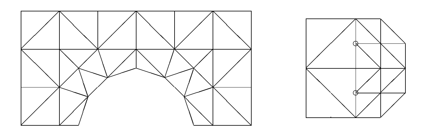
Image (Source: Braess): Left - admissible mesh, right - mesh with "hanging" nodes
Acute and weakly acute triangulations
Definition: A triangulation $\{T_1\dots T_M\}$ of a domain $\Omega$ is
- acute, if all interior angles of all triangles are less than $\frac\pi2$,
- weakly acute, if all interior angles of all triangles are less than or equal to $\frac\pi2$.
Voronoi diagram
After G. F. Voronoi, 1868-1908
Definition: Let $\mathbf p,\mathbf q\in \mathbb R^d$. The set of points $H_{\mathbf p\mathbf q}=\left\{\mathbf x\in \mathbb R^d: ||\mathbf x-\mathbf p||\leq ||\mathbf x-\mathbf q||\right\}$ is the half space of points $\mathbf x$ closer to $\mathbf p$ than to $\mathbf q$.
Definition: Given a finite set of points $S\subset \mathbb R^d$, the Voronoi region (Voronoi cell) of a point $\mathbf p\in S$ is the set of points $\mathbf x$ closer to $\mathbf p$ than to any other point $\mathbf q\in S$: $$V_\mathbf p=\left\{\mathbf x\in \mathbb R^d: ||\mathbf x-\mathbf p||\leq ||\mathbf x-\mathbf q||\,\forall \mathbf q\in S\right\}$$
The Voronoi diagram of $S$ is the collection of the Voronoi regions of the points of $S$.
Voronoi diagram II
- The Voronoi diagram subdivides the whole space into ``nearest neigbor'' regions
- Being intersections of half planes, the Voronoi regions are convex sets
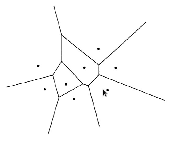
Voronoi diagram of 8 points in the plane (H. Si) \end{minipage}
Delaunay triangulation
After B.N. Delaunay (Delone), 1890-1980
- Given a finite set of points $S\subset \mathbb R^d$
- Assume that the points of $S$ are in general position, i.e. no $d+2$ points of $S$ are on one sphere (in 2D: no 4 points on one circle)
- Connect each pair of points whose Voronoi regions share a common edge with a line
- $\Rightarrow$ Delaunay triangulation of the convex hull of $S$
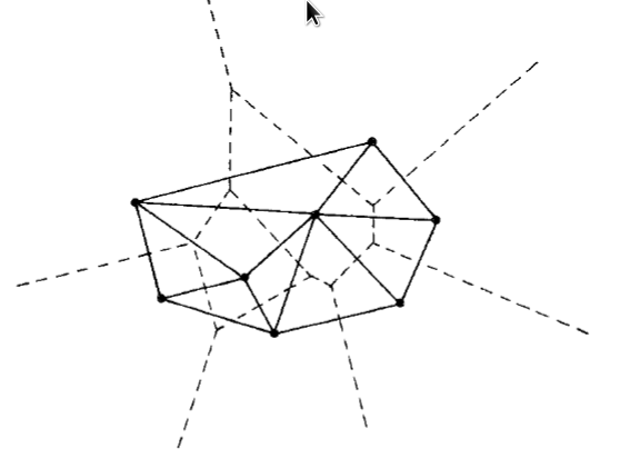
Delaunay triangulation of the convex hull of 8 points in the plane (H.Si)
Interactive example via GEOGRAM
Delaunay triangulation II
- The circumsphere (circumcircle in 2D) of a $d$-dimensional simplex is the unique sphere containing all vertices of the simplex
- The circumball (circumdisc in 2D) of a simplex is the unique (open) ball which has the circumsphere of the simplex as boundary
Definition: A triangulation of the convex hull of a point set $S$ has the Delaunay property if each simplex (triangle) of the triangulation is Delaunay, i.e. its circumsphere (circumcircle) is empty wrt. $S$, i.e. it does not contain any points of $S$.
- The Delaunay triangulation of a point set $S$, where all points are in general position is unique
- Otherwise there is an ambiguity - if e.g. 4 points are one circle, there are two ways to connect them resulting in Delaunay triangles
Edge flips and locally Delaunay edges (2D only)
- For any two triangles $\mathbf a\mathbf b\mathbf c$ and $\mathbf a\mathbf d\mathbf b$ sharing a common edge $\mathbf a\mathbf b$, there is the edge flip operation which reconnects the points in such a way that two new triangles emerge: $\mathbf a\mathbf d\mathbf c$ and $\mathbf c\mathbf d\mathbf b$.
- An edge of a triangulation is locally Delaunay if it either belongs to exactly one triangle, or if it belongs to two triangles, and their respective circumdisks do not contain the points opposite wrt. the edge
- If an edge is locally Delaunay and belongs to two triangles, the sum of the angles opposite to this edge is less or equal to $\pi$.
- If all edges of a triangulation of the convex hull of $S$ are locally Delaunay, then the triangulation is the Delaunay triangulation
- If an edge is not locally Delaunay and belongs to two triangles, the edge emerging from the corresponding edge flip will be locally Delaunay
Lawson's Edge flip algorithm for constructing a Delaunay triangulation
- Input: A stack $L$ of edges of a given triangulation of a set $S$ of $n$ points
- While $L\neq\emptyset$
- pop an edge $\mathbf a\mathbf b$ from $L$
- If $\mathbf a\mathbf b$ is not locally Delaunay
- Flip $\mathbf a\mathbf b$ to $\mathbf c\mathbf d$
- Push edges $\mathbf a\mathbf c,\mathbf c\mathbf b,\mathbf d\mathbf b,\mathbf d\mathbf a$ onto $L$
This algorithm is known to terminate after $O(n^2)$ operations. After termination, all edges will be locally Delaunay, so the output is the Delaunay triangulation of $S$.
- Among all triangulations of a finite point set $S$, the Delaunay triangulation maximises the minimum angle of all triangles2
- The set of all possible triangulations of $S$ is connected via the flip graph. Each edge of this graph corresponds to one particular flip operation
Randomized incremental flip algorithm (2D only)
- Create Delaunay triangulation of point set $S$ by inserting points one after another, and creating the Delaunay triangulation of the emerging subset of $S$ using the flip algorithm
- Estimated complexity: $O(n\log n)$
- In 3D, there is no simple flip algorithm, generalizations are active research subject
Triangle
During this course, we will focus on Triangle. It can be compiled to a standalone executable reading and writing files or to a library which can be called from applications.
Currently in Julia it is accessible as submodule of the package VoronoiFVM.jl. It is planned to become a standalone package, consolidating the use of several Julia packages which already use Triangle.
using Triangulate
using PyPlot
Plot a pair of input and output triangulateio structs
function plotpair(Plotter::Module, triin, triout;voronoi=nothing)
    if Triangulate.ispyplot(Plotter)
        PyPlot=Plotter
        PyPlot.clf()
        PyPlot.subplot(121)
        PyPlot.title("In")
        Triangulate.plot(PyPlot,triin)
        PyPlot.subplot(122)
        PyPlot.title("Out")
        Triangulate.plot(PyPlot,triout,voronoi=voronoi)
    end
end
Delaunay triangulation of the convex hull of a pointset
- Triangle communicates via a data structure
triangulateiowhich contains possible input and output information - It processes an input structure and returns on output the triangulation, and possibly, the Voronoi diagram.
- It is controlled via a string containing switches.
- The switch '-Q' makes Triangle quiet
triin=Triangulate.TriangulateIO()
triin.pointlist=[ 0.0 0; 1 0; 0 1]'
(triout, vorout)=triangulate("", triin)
plotpair(PyPlot,triin,triout)

Additional creation of the convex hull
- The switch '-c' leads to the additional creation of the information about the edges at the convex hull
triin=Triangulate.TriangulateIO()
triin.pointlist=rand(Cdouble,2,7)
(triout, vorout)=triangulate("Qc", triin)
plotpair(PyPlot,triin,triout)

Additional creation of the Voronoi diagram
- The switch '-v' leads to the additional creation of the Voronoi diagram
triin=Triangulate.TriangulateIO()
triin.pointlist=rand(Cdouble,2,7)
(triout, vorout)=triangulate("Qcv", triin)
plotpair(PyPlot,triin,triout,voronoi=vorout)

Conforming Delaunay triangulations
Definition: An admissible triangulation of a polygonal Domain $\Omega\subset \mathbb R^d$ has the boundary conforming Delaunay property if
- All simplices are Delaunay
- All boundary simplices (edges in 2D, facets in 3d) have the Gabriel property, i.e. their minimal circumdisks are empty
Equivalent definition in 2D:
- Sum of angles opposite to interior edges $\leq$ $\pi$,
- angle opposite to boundary edge $\leq \frac\pi2$
Corollary:
- All triangle circumcenters are in the interior of the domain
- Weakly acute triangulations are boundary conforming Delaunay, but not vice versa!
Remarks:
- Working with weakly acute triangulations for general polygonal domains is unrealistic, especially in 3D
- For boundary conforming Delaunay triangulations of polygonal domains there are algoritms with mathematical termination proofs valid in many relevant cases (J. Shewchuk, H. Si)
triin=Triangulate.TriangulateIO()
triin.pointlist=rand(Cdouble,2,7)
(triout, vorout)=triangulate("cv", triin)
plotpair(PyPlot,triin,triout,voronoi=vorout)

Boundary conforming Delaunay triangulation of convex hull
- The switch '-D' leads to the creation of a boundary conforming Delaunay triangulation.
- In this case, "Steiner points" need to be added to the initial point set
triin=Triangulate.TriangulateIO()
triin.pointlist=rand(Cdouble,2,7)
(triout, vorout)=triangulate("Dcv", triin)
plotpair(PyPlot,triin,triout,voronoi=vorout)

Triangulations of finite polygonal domains
- So far, we discussed triangulations of point sets which at best can describe convex domains
- Create Delaunay triangulation of point set, "add" segments of a Piecewise Linear Straight Line Graph (PLSG) describing the boudary of the domain. This results in a "constrained Delaunay triangulation" which may not have the Delaunay property with respect to the bundary vertices.
- Domain is specfied as a piecewise linear straight line graph
- In addition to the point list, we give a list of segments, and use "-p" instead of "-c"
- An additional segement marker list can be specified
triin=Triangulate.TriangulateIO()
triin.pointlist=Matrix{Cdouble}([0.0 0.0 ; 1.0 0.0 ; 0.4  0.4 ; 0.0 1.0; 0.2 0.3]')
triin.segmentlist=Matrix{Cint}([1 2 ; 2 3 ; 3 4 ; 4 1 ]')
triin.segmentmarkerlist=Vector{Int32}([1, 2, 3, 4])
(triout, vorout)=triangulate("pv", triin)
plotpair(PyPlot,triin,triout,voronoi=vorout)

Boundary conforming Delaunay triangulation
- Once again, '-D' adds the boundary conforming Delaunay property
triin=Triangulate.TriangulateIO()
triin.pointlist=Matrix{Cdouble}([0.0 0.0 ; 1.0 0.0 ; 0.4  0.4 ; 0.0 1.0; 0.2 0.3]')
triin.segmentlist=Matrix{Cint}([1 2 ; 2 3 ; 3 4 ; 4 1 ]')
triin.segmentmarkerlist=Vector{Int32}([1, 2, 3, 4])
(triout, vorout)=triangulate("pvD", triin)
plotpair(PyPlot,triin,triout,voronoi=vorout)

Domain triangulation with area constraint
- '-a' allows to specify a maximum area constraint.
- '-q' allows to specify minumum angle
triin=Triangulate.TriangulateIO()
triin.pointlist=Matrix{Cdouble}([0.0 0.0 ; 1.0 0.0 ; 0.4  0.4 ; 0.0 1.0; 0.2 0.3]')
triin.segmentlist=Matrix{Cint}([1 2 ; 2 3 ; 3 4 ; 4 1 ]')
triin.segmentmarkerlist=Vector{Int32}([1, 2, 3, 4])
(triout, vorout)=triangulate("pa0.1", triin)
plotpair(PyPlot,triin,triout,voronoi=vorout)

Domain triangulation with area constraint from user function
- '-u' allows to specify a user defined refinement criterion
- Julia constructs a c-callable function which is called by Triangle
function unsuitable(x1,y1,x2,y2,x3,y3,area)
    bary_x=(x1+x2+x3)/3.0
    bary_y=(y1+y2+y3)/3.0
    dx=bary_x-0.1
    dy=bary_y-0.1
    area>0.001*exp(50.0*(dx^2+dy^2))
end
triin=Triangulate.TriangulateIO()
triin.pointlist=Matrix{Cdouble}([0.0 0.0 ; 1.0 0.0 ; 0.4  0.4 ; 0.0 1.0; 0.2 0.3]')
triin.segmentlist=Matrix{Cint}([1 2 ; 2 3 ; 3 4 ; 4 1 ]')
triin.segmentmarkerlist=Vector{Int32}([1, 2, 3, 4])
triunsuitable(unsuitable)
(triout, vorout)=triangulate("pa0.1u", triin)
plotpair(PyPlot,triin,triout,voronoi=vorout)

Relevant output for numerical simulation (depends on method, implementation $\dots$):
- List of points
- List of triangles which for each triangle describes indices of points belonging to triangle
- List of (boundary) segments which for each segment describes indices of points belonging to segment
- Possibly: list of segment markers (which can be used to distiguish boundary conditions)
- Possibly: list of triangle attributes (which describe subdomain information)
triin=Triangulate.TriangulateIO()
triin.pointlist=Matrix{Cdouble}([0.0 0.0 ; 1.0 0.0 ; 0.4  0.4 ; 0.0 1.0; 0.2 0.3]')
triin.segmentlist=Matrix{Cint}([1 2 ; 2 3 ; 3 4 ; 4 1 ]')
triin.segmentmarkerlist=Vector{Int32}([1, 2, 3, 4])
(triout, vorout)=triangulate("pa0.1Q", triin)
plotpair(PyPlot,triin,triout,voronoi=vorout)

@show triout.pointlist
@show triout.trianglelist
@show triout.segmentlist
@show triout.segmentmarkerlist
@show triout.triangleattributelist
This notebook was generated using Literate.jl.