Scientific Computing, TU Berlin, WS 2019/2020, Lecture 05
Jürgen Fuhrmann, WIAS Berlin
Solution of linear systems of equations
- Let $A$ be an $N \times N$ matrix, $b\in \mathbb R^N$.
- Solve $Ax=b$
Direct methods
- Exact up to machine precision (see condition number problem...)
- Expensive (in time and space) depending on matrix properties
Iterative methods
- "Only" approximate
- with good convergence and proper accuracy control, results may be not worse than for direct methods
- May be cheaper in space and (possibly) time
- Convergence guarantee is problem dependent and can be tricky
Complexity: "big O notation"
Let $f,g: \mathbb V \to \mathbb R^+$ be some functions, where $\mathbb V=\mathbb N$ or $\mathbb V=\mathbb R$.
Write $$f(x)=O(g(x)) \quad (x\to\infty)$$ if there exist a constant $C>0$ and $x_0\in \mathbb V$ such that $$ \forall x>x_0, \quad |f(x)|\leq C|g(x)|$$
Often, one skips the part "$(x \to \infty)$"
Examples:
- Addition of two vectors: $O(N)$
- Matrix-vector multiplication (for matrix where all entriesre assumed to be nonzero): $O(N^2)$
Really bad example of direct method:
Solve $Ax=b$ by Cramer's rule
\begin{align*} x_i=\left| \begin{matrix} a_{11}&a_{12}&\ldots&a_{1i-1}&b_1&a_{1i+1}&\ldots&a_{1N}\\ a_{21}& &\ldots& &b_2& &\ldots&a_{2N}\\ \vdots& & & &\vdots& & &\vdots\\ a_{N1}& &\ldots& &b_N& &\ldots&a_{NN} \end{matrix}\right| / |A| \quad (i=1\dots N) \end{align*}
This takes $O(N!)$ operations...
Gaussian elimination
- Essentially the only feasible direct solution method
- Solve $Ax=b$ with square matrix $A$.
- While formally, the algorithm is always the same, its implementation depends on
- data structure to store matrix
- possibility to ignore zero entries for matrices with many zeroes
- sorting of elements
Pass 1
\begin{align*} \left( \begin{matrix} 6&-2 &2\\ 12&-8 &6\\ 3 &-13&3 \end{matrix}\right) x= \left(\begin{matrix} 16\\ 26\\ -19 \end{matrix}\right) \end{align*}Step 1: $\mathrm{eqn}_2 \leftarrow \mathrm{eqn}_2-2\,\mathrm{eqn}_1$, $\mathrm{eqn}_3 \leftarrow \mathrm{eqn}_3-\frac12\,\mathrm{eqn}_1$
\begin{align*} \left(\begin{matrix} 6&-2 &2\\ 0 &-4 &2\\ 0 &-12&2 \end{matrix} \right) x= \left(\begin{matrix} 16\\ -6\\ -27 \end{matrix}\right) \end{align*}Step 2: $\mathrm{eqn}_3 \leftarrow \mathrm{eqn}_3-3\,\mathrm{eqn}_2$ \begin{align*} \left(\begin{matrix} 6&-2 &2\\ 0 &-4 &2\\ 0 & 0&-4 \end{matrix}\right) x= \left(\begin{matrix} 16\\ -6\\ -9 \end{matrix}\right) \end{align*}
Pass 2
Solve upper triangular system \begin{align*} \left(\begin{matrix} 6&-2 &2\\ 0 &-4 &2\\ 0 &0&-4 \end{matrix}\right) x= \left(\begin{matrix} 16\\ -6\\ -9 \end{matrix}\right) \end{align*} \begin{align*} -4 x_3&= -9 &&&\Rightarrow x_3&= \frac94\\ -4 x_2 + 2 x_3 &= -6 &\Rightarrow -4 x_2 &= -\frac{21}{2} & \Rightarrow x_2&=\frac{21}{8}\\ 6x_1 -2 x_2 + 2 x_3 &= 2 &\Rightarrow 6x_1 &= 2+ \frac{21}{4}-\frac{18}{4}=\frac{11}{4} & \Rightarrow x_1&=\frac{11}{4}\\ \end{align*}
Interpretation in matrix notation
Pass 1 expressed in matrix operation \begin{align*} L_1Ax= \left(\begin{matrix} 6&-2 &2\\ 0 &-4 &2\\ 0 &-12&2 \end{matrix}\right) x&= \left(\begin{matrix} 16\\ -6\\ -27 \end{matrix}\right) =L_1 b, & L_1&= \left(\begin{matrix} 1&0&0\\ -2&1&0\\ -\frac12&0&1 \end{matrix}\right) \end{align*}\begin{align*} L_2L_1Ax= \left(\begin{matrix} 6&-2 &2\\ 0 &-4 &2\\ 0 & 0&-4 \end{matrix}\right) x&= \left(\begin{matrix} 16\\ -6\\ -9 \end{matrix}\right) =L_2L_1 b, & L_2&= \left(\begin{matrix} 1&0&0\\ 0&1&0\\ 0&-3&1 \end{matrix}\right) \end{align*}
- Let $L=L_1^{-1}L_2^{-1}= \left(\begin{matrix} 1&0&0\\ 2&1&0\\ \frac12&3&1 \end{matrix}\right)$, $U= L_2L_1A$. Then $A=LU$
- Inplace operation: diagonal elements of $L$ are always 1, so no need to store them $\Rightarrow$ work on storage space for $A$ and overwrite it.
LU factorization
Solve $Ax=b$:
- Pass 1: factorize $A=LU$ such that $L,U$ are lower/upper triangular
- Pass 2: obtain $ x=U^{-1}L^{-1}b$ by solution of lower/upper triangular systems
- solve $L\tilde x=b$
- solve $Ux=\tilde x$
A problem for LU factorization
- Consider
- Solution: $\left(\begin{matrix} x_1\\ x_2 \end{matrix}\right) =\left(\begin{matrix} 1\\1 \end{matrix}\right)$
- Machine arithmetic: Let $\epsilon << 1$ such that $1+\epsilon=1$.
- Equation system in machine arithmetic: \begin{align*} 1\cdot\epsilon + 1\cdot 1 &= 1+\epsilon\\ 1\cdot 1 + 1\cdot 1 &=2 \end{align*}
using LinearAlgebra
ϵ=1.0e-5
A=[ϵ 1 ; 1 1]
x=[1,1]
b=[1,2]
@show A*x-b
- Ordinary elimination: $\mathrm{eqn}_2 \leftarrow \mathrm{eqn}_2 - \frac1\epsilon \; \mathrm{eqn}_1$
- In exact arithmetic:
- In floating point arithmetic: $1+\epsilon=1$, $1-\frac1\epsilon=-\frac1\epsilon$, $2-\frac1\epsilon=-\frac1\epsilon$:
$\Rightarrow$ $x_2=1$ $\Rightarrow$ $\epsilon x_1 +1 =1$ $\Rightarrow$ $x_1=0$
ϵ=1.0e-5
A=[ϵ 1 ; 0 1-1/ϵ]
x=[1,1]
b=[1+ϵ,2-(1+ϵ)/ϵ]
@show A*x-b;
Partial Pivoting
- Before elimination step, look at the element with largest absolute value in current column and put the corresponding row
on top'' as thepivot'' - This prevents near zero divisions and increases stability
- Independent of $\epsilon$: \begin{align*} x_2=\frac{1-\epsilon}{1-\epsilon}=1,\qquad x_1=2-x_2=1 \end{align*}
ϵ=1.0e-5
A=[1 1 ; 0 1-ϵ]
x=[1,1]
b=[2,1-ϵ]
@show A*x-b;
- Instead of $A$, factorize $PA$: $PA=LU$, where $P$ is a permutation matrix which can be encoded using an integer vector
How does Julia handle the LU factorization ?
ϵ=1.0e-5
A=[ϵ 1 ; 1 1]
b=[1,2]
x=A\b
@show x;
@show A*x-b;
It seems it does something right ...
Alu=lu(A)
LxU=Alu.L*Alu.U
@show LxU
@show LxU[Alu.p,:]
@show Alu.p
- The LU factorization object has three components: L, U, and p: the two factors and the pivot table
Gaussian elimination and LU factorization
- Full pivoting: in addition to row exchanges, perform column exchanges to ensure even larger pivots. Seldomly used in practice.
- Gaussian elimination with partial pivoting is the "working horse" for direct solution methods
- Complexity of LU-Factorization: $O(N^3)$, some theoretically better algorithms are known with e.g. $O(N^{2.736})$
- Complexity of triangular solve: $O(N^2)$ $\Rightarrow$ overall complexity of linear system solution is $O(N^3)$
- Cholesky factorization: $A=LL^T$ for symmetric, positive definite matrices
Implementation
- Due to multiple dispatch Julia chooses the best implementation for a given data type
- Generic variant for any number typpe
BLAS, LAPACK for Float32, Float64
BLAS: Basic Linear Algebra Subprograms (http://www.netlib.org/blas/)
- Level 1 - vector-vector: $\mathbf{y} \leftarrow \alpha \mathbf{x} + \mathbf{y}$
- Level 2 - matrix-vector: $\mathbf{y} \leftarrow \alpha A \mathbf{x} + \beta \mathbf{y}$
- Level 3 - matrix-matrix: $C \leftarrow \alpha A B + \beta C$
LAPACK: Linear Algebra PACKage (http://www.netlib.org/lapack/)
- Linear system solution, eigenvalue calculation etc.
dgetrf: LU factorizationdgetrs: LU solve
Used in overwhelming number of codes (e.g. matlab, scipy etc.). Also, C++ matrix libraries use these routines. Unless there is special need, they should be used.
- Reference implementations in Fortran, but many more implementations available which carefully work with cache lines etc.
Matrices from Partial Differential Equations (PDEs)
- So far, we assumed that matrices are stored in a two-dimensional, $N\times N$ array of numbers
- This kind of matrix storage are also called dense
- As we will see, matrices from PDEs (can) have a number of structural properties one can take advantage of when storing a matrix and solving the linear system
1D heat conduction
- $v_L, v_R$: ambient temperatures, $\alpha$: heat transfer coefficient
- Second order boundary value problem in $\Omega=[0,1]$: \begin{align*} -u''(x)&=f(x) &\text{in} \Omega\\ -u'(0) + \alpha (u(0) - v_L)&=0\\ u'(1) + \alpha (u(1) - v_R)&=0 \end{align*}
- Let $h=\frac1{N-1}$, $x_i=x_0+(i-1)h$ ($i=1\dots n$) be discretization points, let $u_i$ approximations for $u(x_i)$ and $f_i=f(x_i)$
- Finite difference approximation: \begin{align*} -u'(0) +\alpha (u(0) - v_L) &\approx \frac{1}{h}(u_{0}-u_1) + \alpha (u_0 - v_L) \\ -u''(x_i)-f(x_i) &\approx \frac{1}{h^2}(-u_{i+1}+2u_i- u_{i-1})-f_i & (i=2\dots N-1)\\ u'(1) + \alpha (u(1) - v_R) &\approx \frac{1}{h}(u_{N}-u_{N-1})+ \alpha (u_N - v_R)\\ \end{align*}
1D heat conduction: discretization matrix}
- equations $2\dots N-1$ multiplied by $h$
- only nonzero entries written
- Each row contains $\leq 3$ elements
- Only $3N-2$ of $N^2$ elements are non-zero
General tridiagonal matrix
\begin{align*} \left(\begin{matrix} {b_1} & {c_1} & { } & { } & { } \\ {a_2} & {b_2} & {c_2} & { } & { } \\ { X} & {a_3} & {b_3} & \ddots & { } \\ { } & { } & \ddots & \ddots & {c_{n-1}}\\ { } & { } & { } & {a_N} & {b_N}\\ \end{matrix}\right) \left(\begin{matrix} {u_1 } \\ {u_2 } \\ {u_3 } \\ \vdots \\ {u_N } \\ \end{matrix}\right) = \left(\begin{matrix} {f_1 } \\ {f_2 } \\ {f_3 } \\ \vdots \\ {f_N } \\ \end{matrix}\right) \end{align*}- To store matrix, it is sufficient to store only nonzero elements in three one-dimensional arrays for $a_i, b_i, c_i$, respectively
Gaussian elimination for tridiagonal systems
Gaussian elimination using arrays $a,b,c$ as matrix storage ?
- From what we have seen, this question arises in a quite natural way, and historically, the answer has been given several times and named differently
- TDMA (tridiagonal matrix algorithm)
- "Thomas algorithm" (Llewellyn H. Thomas, 1949 (?))
- "Progonka method" (from Russian "progonka" "run through"; Gelfand, Lokutsievski, 1952, published 1960)
Progonka: derivation
- $a_i u_{i-1} + b_i u_i + c_i u_{i+1} = f_i \quad (i=1\dots N)$; $a_1=0$, $c_N=0$
- For $i=1\dots N-1$, assume there are coefficients $\alpha_i, \beta_i$ such that $u_i=\alpha_{i+1}u_{i+1}+\beta_{i+1}$.
- Then, we can express $u_{i-1}$ and $u_{i}$ via $u_{i+1}$: $$(a_i\alpha_i\alpha_{i+1}+ b_i \alpha_{i+1} + c_i) u_{i+1} + a_i\alpha_i\beta_{i+1}+ a_i\beta_i +b_i \beta_{i+1} -f_i=0$$
- This is true independently of $u$ if
- or for $i=1\dots N-1$:
Progonka: realization
Initialization: $\begin{cases} \alpha_{2}&= -\frac{c_1}{b_1}\\ \beta_{2} &= \frac{f_i}{b_1} \end{cases}$
Forward sweep: for $i=2\dots N-1$: $\begin{cases} \alpha_{i+1}&= -\frac{c_i}{a_i\alpha_i+b_i}\\ \beta_{i+1} &= \frac{f_i - a_i\beta_i}{a_i\alpha_i+b_i} \end{cases}$
$u_N=\frac{f_N - a_N\beta_N}{a_N\alpha_N+b_N}$
- Backward sweep: for $i= N-1 \dots 1$: $u_i=\alpha_{i+1}u_{i+1}+\beta_{i+1}$
Прогонка: properties
- $n$ unknowns, one forward sweep, one backward sweep $\Rightarrow$ $O(N)$ operations vs. $O(N^3)$ for algorithm using full matrix
- No pivoting $\Rightarrow$ stability issues
- Stability for diagonally dominant matrices ($|b_i| > |a_i| + |c_i|$)
- Stability for symmetric positive definite matrices
Progonka: Julia
Diagonally dominant matrix
N=5
a=[0.1 for i=1:N-1]
b=[0.5 for i=1:N]
c=[0.1 for i=1:N-1]
A=Tridiagonal(a,b,c)
Alu=lu(A)
@show Alu.p
@show Alu.L*Alu.U
rhs=[1.0 for i=1:N]
x=A\rhs
@show A*x-rhs
Random matrix $\Rightarrow$ pivoting
a=randn(N-1)
b=randn(N)
c=randn(N-1)
A=Tridiagonal(a,b,c)
Alu=lu(A)
@show Alu.p
@show Alu.L*Alu.U
rhs=[1.0 for i=1:N]
x=A\rhs
@show A*x-rhs
used dgtrsv from LAPACK
2D Rectangular discretization grid
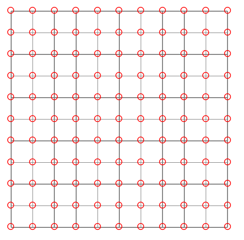
- Each discretization point has not more then 4 neighbours
- Matrix can be stored in five diagonals, LU factorization not anymore $\equiv$ "fill-in"
- Certain iterative methods can take advantage of the regular and hierachical structure (multigrid) and are able to solve system in $O(N)$ operations
- Another possibility: fast Fourier transform with $O(N\log N)$ operations
Sparse matrices
- Tridiagonal and five-diagonal matrices can be seen as special cases of sparse matrices
- Generally they occur in finite element, finite difference and finite volume discretizations of PDEs on structured and unstructured grids
- Definition: Regardless of number of unknowns $N$, the number of non-zero entries per row remains limited by $n_r$
- If we find a scheme which allows to store only the non-zero matrix entries, we would need $Nn_r= O(N)$ storage locations instead of $N^2$
- The same would be true for the matrix-vector multiplication if we program it in such a way that we use every nonzero element just once: matrix-vector multiplication would use $O(N)$ instead of $O(N^2)$ operations
Sparse matrix formats
- What is a good storage format for sparse matrices?
- Is there a way to implement Gaussian elimination for general sparse matrices which allows for linear system solution with $O(N)$ operation ?
- Is there a way to implement Gaussian elimination \emph{with pivoting} for general sparse matrices which allows for linear system solution with $O(N)$ operations?
- Is there any algorithm for sparse linear system solution with $O(N)$ operations?
Coordinate (triplet) format
- Store all nonzero elements along with their row and column indices
- One real, two integer arrays, length = nnz= number of nonzero elements
 Y.Saad, Iterative Methods, p.92}
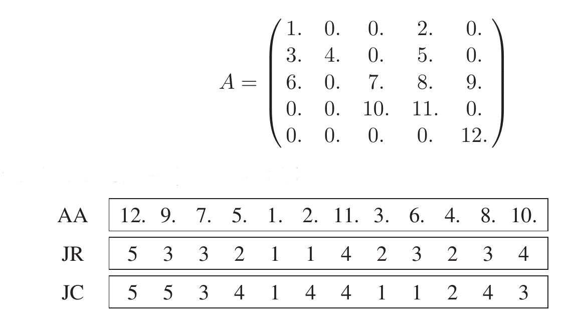
Compressed Row Storage (CRS) format}
(aka Compressed Sparse Row (CSR) or IA-JA etc.)
- real array
AA, length nnz, containing all nonzero elements row by row - integer array
JA, length nnz, containing the column indices of the elements ofAA - integer array
IA, length N+1, containing the start indizes of each row in the arraysIAandJAandIA[N+1]=nnz+1\begin{align*} A&= \left(\begin{matrix} 1.& 0. & 0.& 2.& 0.\\ 3.& 4. & 0.& 5.& 0.\\ 6.& 0. & 7.& 8.& 9.\\ 0.& 0. & 10.& 11. & 0.\\ 0.& 0. & 0.& 0.& 12. \end{matrix}\right)\\ \end{align*}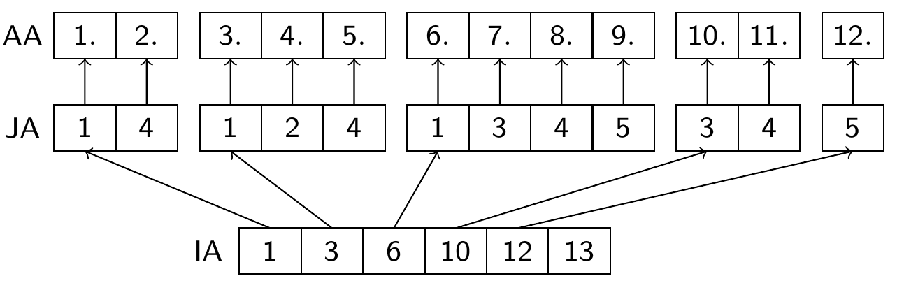
- Used in most sparse matrix solver packages
- CSC (Compressed Column Storage) uses similar principle but stores the matrix column-wise. Used in Julia
Sparse direct solvers
- Sparse direct solvers implement Gaussian elimination with different pivoting strategies
- UMFPACK: Used in Julia
- Pardiso (omp + MPI parallel)
- SuperLU (omp parallel)
- MUMPS (MPI parallel)
- Pastix
- Quite efficient for 1D/2D problems
- Essentially they implement the LU factorization algorithm
- They suffer from fill-in, especially for 3D problems: Let $A=LU$ be an LU-Factorization. Then, as a rule, $nnz(L+U) > nnz(A)$.
- $\Rightarrow$ increased memory usage to store L,U
- $\Rightarrow$ high operation count
Sparse direct solvers: solution steps (Saad Ch. 3.6)
- Pre-ordering
- Decrease amount of non-zero elements generated by fill-in by re-ordering of the matrix
- Several, graph theory based heuristic algorithms exist
- Symbolic factorization
- If pivoting is ignored, the indices of the non-zero elements are calculated and stored
- Most expensive step wrt. computation time
- Numerical factorization
- Calculation of the numerical values of the nonzero entries
- Moderately expensive, once the symbolic factors are available
- Upper/lower triangular system solution
- Fairly quick in comparison to the other steps
- Separation of steps 2 and 3 allows to save computational costs for problems where the sparsity structure remains unchanged, e.g. time dependent problems on fixed computational grids
- With pivoting, steps 2 and 3 have to be performed together, and pivoting can increase fill-in
- Instead of pivoting, iterative refinement may be used in order to maintain accuracy of the solution
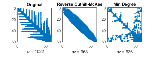
Sparse direct solvers: influence of reordering
- Sparsity patterns for original matrix with three different orderings of unknowns
- number of nonzero elements (of course) independent of ordering:
 (mathworks.com)
- number of nonzero elements (of course) independent of ordering:
- Sparsity patterns for corresponding LU factorizations
- number of nonzero elements depend original ordering!
 (mathworks.com)
- number of nonzero elements depend original ordering!
Sparse direct solvers: Complexity estimate
- Complexity estimates depend on storage scheme, reordering etc.
- Sparse matrix - vector multiplication has complexity $O(N)$
- Some estimates can be given from graph theory for discretizations of heat equation with $N=n^d$ unknowns on close to cubic grids in space dimension $d$
- sparse LU factorization:
- triangular solve: work dominated by storage complexity
(Source: J. Poulson, PhD thesis, http://hdl.handle.net/2152/ETD-UT-2012-12-6622)
Julia code
using SparseArrays
N=100
A=sprand(N,N,0.5) # random matrix with probaility 0.5 that $A_{ij}$ is nonzero
Alu=lu(A)
@show Alu.p
b=ones(N)
x=A\b
@show norm(A*x-b)
using Plots
@show nnz(A)
spy(A)
LxU=Alu.L*Alu.U
@show nnz(LxU)
spy(LxU)
This notebook was generated using Literate.jl.