[Next]:  A descent method for the free  
 [Up]:  Projects  
 [Previous]:  Calculation of electronic band structure of  
 [Contents]   [Index] 


Modeling, analysis and simulation of mode-locked semiconductor lasers

Collaborator: U. Bandelow (FG 1), A. Vladimirov

 (FG 2)

Cooperation with: B. Hüttl, R. Kaiser, (Fraunhofer-Institut für Nachrichtentechnik, Heinrich-Hertz-Institut (HHI), Berlin)

Supported by: Terabit Optics Berlin (project B4)

Description:

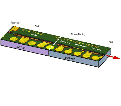
Mode-locked semiconductor lasers have attracted considerable research interest for many years, for their high speed potential as well as the possible generation of intense pulses. Together with our partners, we are aiming at an optical data transmission at rates of 40 GHz. A typical device under consideration is sketched in Figure 1.

Fig. 1: Monolithic multisection DBR laser as fabricated at HHI Berlin. It consists of a reversely biased saturable absorber section, a forward biased gain section, a passive phase tuning section, and a passive distributed Bragg reflector (DBR) section and is designed for emission of pulse trains with 40 GHz repetition frequency.
\ProjektEPSbildNocap{0.6\textwidth}{ml-laser_uwe1}

In a mode-locked laser, a spatio-temporal structure develops across the entire device, which has to be properly accounted for. An adequate description is given by the traveling wave equations (TWE)

$\displaystyle \left(\vphantom{ -\frac{i}{v_{g}} \frac{\partial }{\partial t}\mp i\frac{\partial }{%
\partial z}+\beta }\right.$ - $\displaystyle {\frac{{i}}{{v_{g}}}}$ $\displaystyle {\frac{{\partial}}{{\partial t}}}$$\displaystyle \mp$i$\displaystyle {\frac{{\partial }}{{%
\partial z}}}$ + $\displaystyle \beta$$\displaystyle \left.\vphantom{ -\frac{i}{v_{g}} \frac{\partial }{\partial t}\mp i\frac{\partial }{%
\partial z}+\beta }\right)$E$\scriptstyle \pm$ + $\displaystyle \kappa$E$\scriptstyle \mp$ = 0 (1)
for the slowly varying amplitudes E+(z, t) and E-(z, t) of the forward and back traveling waves, respectively. The boundary conditions are E-(L, t) = rLE+(L, t) and E+(0, t) = r0E-(0, t) at the facets of the laser. $ \beta$ is a function of the locally distributed carrier density n(z, t), which itself is governed by

$\displaystyle \partial_{{t}}^{}$n = J(z, t) - R$\displaystyle \left(\vphantom{ n}\right.$n$\displaystyle \left.\vphantom{ n}\right)$ - vg $\displaystyle \Re$e[E * (g + 2$\displaystyle \mathcal {D}$)E]. (2)
Especially in the absorber and the gain section, the model for $ \beta$ is

$\displaystyle \beta$ = - i$\displaystyle {\frac{{\alpha }}{{2}}}$ + (i + $\displaystyle \alpha_{{H}}^{}$)$\displaystyle {\frac{{g}}{{2}}}$ + i$\displaystyle \mathcal {D}$   (active sections), (3)
where the gain g also depends on n. $ \mathcal {D}$ is a dispersion operator defined by
$\displaystyle \mathcal {D}$E$\scriptstyle \pm$ $\displaystyle \overset{def}{=}$ $\displaystyle {\frac{{\bar{g}}}{{2}}}$(E$\scriptstyle \pm$ - p$\scriptstyle \pm$)      and      (4)
- i$\displaystyle \partial_{{t}}^{}$p$\scriptstyle \pm$ = - i$\displaystyle \bar{{\gamma}}$(E$\scriptstyle \pm$ - p$\scriptstyle \pm$) + $\displaystyle \bar{{\omega}%
}$p$\scriptstyle \pm$. (5)

More details can be found in [1]. The above distributed time-domain model will be in the following shortly referred to as the TWE model. In practise, we use this TWE model for numerical simulation (LDSL) and quantitative comparison with the experiment.

Fig. 2: Typical simulation results obtained with LDSL-tool on mode-locked lasers. Stable mode locking occurs in the shaded areas where also the repetition frequencies are given. Outside these areas, mode locking becomes unstable: Supermodulation by slower Q-switching as well as multiple pulses can appear.
\ProjektEPSbildNocap{0.5\textwidth}{area_scheme}

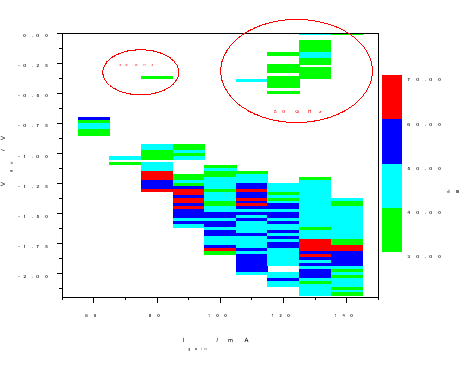
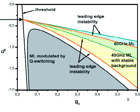
Typical simulation results are schematically drawn in Figure 2. As indicated there, other effects occur outside the mode-locking areas which hinder applications. These effects influence smoothly the mode-locking behavior already within the shaded areas, resulting in an increasing amplitude noise, if one approaches the boundaries. Above the 40-GHz area, we discovered a region where a two-pulse (instead of one) scenario appears.

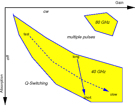
To our surprise, we observed the stabilization of the two pulses when we decreased the absorption even more and increased the gain slightly, thereby approaching the upper right area in Figure 2 called 80 GHz. In this situation the two pulses keep the maximum distance in the resonator and counter-propagate through it. This is indicated by the completely correlated output pulses at the two end facets, drawn in the upper Figure 3, with a repetition frequency of 80 GHz. The latter is twice the roundtrip frequency, such that we can call it harmonic mode locking. The surprising thing is that there is no specific geometrical construction as, e.g., a ring resonator or a colliding pulse scheme which would support this type of mode locking: The pulses meet simply somewhere in the phase tuning section without specifically gaining from that. The harmonic mode locking appears to be self-starting and is stable over a finite range of parameters. So far, this was our first observation from numerical simulations with the TWE model. Later in 2004, this phenomenon has, indeed, been measured at the HHI with autocorrelation techniques. The measured autocorrelation trace is depicted in the lower Figure 3 and displays a periodic signal with a repetition frequency of 80 GHz, which corresponds to our prediction.

Fig. 3: 80-GHz mode locking. Upper: Time trace of output power at both facets of the harmonic mode-locked laser, prediction by simulation. Lower: Measured autocorellation trace.
\makeatletter
\@ZweiProjektbilderNocap[v]{0.5\textwidth}{80GHz_ldsl}{80GHz_auto_hhi}
\makeatother

Even more, the harmonic mode locking has been measured in the same region of parameters as predicted by the theory, cf. shaded ``80 GHz'' areas in Figure 2 and in Figure 4.

Fig. 4: Mode-locking areas incl. 80 GHz harmonic mode locking, measured at HHI
\ProjektEPSbildNocap{0.55\textwidth}{80GHz_area_hhi}

For a qualitative analysis, we use in addition lumped differential-delay models [2], similar to the Lang-Kobayashi treatment of lasers with external feedback. When deriving these models, we do not use the approximations of small gain and loss per cavity round trip and weak saturation. Therefore, our models are capable of describing mode locking in the parameter range of semiconductor lasers. In the first, ring cavity model, the equations governing the time evolution of the electric field amplitude a(t) at the entrance of the gain section, saturable gain g(t), and saturable loss q(t) take the form of delay differential equations, [2, 3],

$\displaystyle \gamma^{{-1}}_{}$$\displaystyle \partial_{{t}}^{}$a$\displaystyle \left(\vphantom{ t }\right.$t$\displaystyle \left.\vphantom{ t }\right)$ + a$\displaystyle \left(\vphantom{ t }\right.$t$\displaystyle \left.\vphantom{ t }\right)$ = $\displaystyle \sqrt{{\xi }}$e$\scriptstyle \left(\vphantom{ 1-i\alpha _{H2}}\right.$1 - i$\scriptstyle \alpha_{{H2}}$$\scriptstyle \left.\vphantom{ 1-i\alpha _{H2}}\right)$g$\scriptstyle \left(\vphantom{ t -T}\right.$t - T$\scriptstyle \left.\vphantom{ t -T}\right)$/2-$\scriptstyle \left(\vphantom{ 1-i\alpha _{H1}}\right.$1 - i$\scriptstyle \alpha_{{H1}}$$\scriptstyle \left.\vphantom{ 1-i\alpha _{H1}}\right)$q$\scriptstyle \left(\vphantom{ t -T}\right.$t - T$\scriptstyle \left.\vphantom{ t -T}\right)$/2+i$\scriptstyle \phi$a$\displaystyle \left(\vphantom{
t -T}\right.$t - T$\displaystyle \left.\vphantom{
t -T}\right)$, (6)

$\displaystyle \partial_{{t}}^{}$q$\displaystyle \left(\vphantom{ t }\right.$t$\displaystyle \left.\vphantom{ t }\right)$ = - q0 - $\displaystyle {\frac{{q\left( t \right) }}{{%
\tau _{1}}}}$ - s$\displaystyle \left(\vphantom{ 1-e^{-q\left( t \right) }}\right.$1 - e-q$\scriptstyle \left(\vphantom{ t }\right.$t$\scriptstyle \left.\vphantom{ t }\right)$$\displaystyle \left.\vphantom{ 1-e^{-q\left( t \right) }}\right)$$\displaystyle \left\vert\vphantom{ A\left(
t \right) }\right.$A$\displaystyle \left(\vphantom{ t }\right.$t$\displaystyle \left.\vphantom{ t }\right)$$\displaystyle \left.\vphantom{ A\left(
t \right) }\right\vert^{{2}}_{}$, (7)

$\displaystyle \partial_{{t}}^{}$g$\displaystyle \left(\vphantom{ t }\right.$t$\displaystyle \left.\vphantom{ t }\right)$ = g0 - $\displaystyle {\frac{{g\left( t \right) }}{{%
\tau _{2}}}}$ - e-q$\scriptstyle \left(\vphantom{ t }\right.$t$\scriptstyle \left.\vphantom{ t }\right)$$\displaystyle \left(\vphantom{ e^{g\left( t \right)
}-1}\right.$eg$\scriptstyle \left(\vphantom{ t }\right.$t$\scriptstyle \left.\vphantom{ t }\right)$ - 1$\displaystyle \left.\vphantom{ e^{g\left( t \right)
}-1}\right)$$\displaystyle \left\vert\vphantom{ A\left(
t \right) }\right.$A$\displaystyle \left(\vphantom{ t }\right.$t$\displaystyle \left.\vphantom{ t }\right)$$\displaystyle \left.\vphantom{ A\left(
t \right) }\right\vert^{{2}}_{}$. (8)
The second, linear cavity model, assumes that both gain and saturable absorber sections are thin as compared to the pulse width. In the case when the absorber section is situated close to one of the two cavity mirrors, this model takes the form:

$\displaystyle \gamma^{{-1}}_{}$$\displaystyle \partial_{{t}}^{}$a$\displaystyle \left(\vphantom{ t }\right.$t$\displaystyle \left.\vphantom{ t }\right)$ + a$\displaystyle \left(\vphantom{ t }\right.$t$\displaystyle \left.\vphantom{ t }\right)$ = $\displaystyle \sqrt{{\xi
_{1}\xi _{2}}}$e$\scriptstyle \left(\vphantom{ 1-i\alpha _{H2}}\right.$1 - i$\scriptstyle \alpha_{{H2}}$$\scriptstyle \left.\vphantom{ 1-i\alpha _{H2}}\right)$$\scriptstyle \left[\vphantom{ g\left(
t-T\right) +g\left( t-T+\tau \right) }\right.$g$\scriptstyle \left(\vphantom{ t -T}\right.$t - T$\scriptstyle \left.\vphantom{ t -T}\right)$ + g$\scriptstyle \left(\vphantom{ t-T+\tau }\right.$t - T + $\scriptstyle \tau$$\scriptstyle \left.\vphantom{ t-T+\tau }\right)$$\scriptstyle \left.\vphantom{ g\left(
t-T\right) +g\left( t-T+\tau \right) }\right]$/2-$\scriptstyle \left(\vphantom{ 1-i\alpha _{H1}}\right.$1 - i$\scriptstyle \alpha_{{H1}}$$\scriptstyle \left.\vphantom{ 1-i\alpha _{H1}}\right)$q$\scriptstyle \left(\vphantom{ t -T}\right.$t - T$\scriptstyle \left.\vphantom{ t -T}\right)$+i$\scriptstyle \phi$a$\displaystyle \left(\vphantom{
t -T}\right.$t - T$\displaystyle \left.\vphantom{
t -T}\right)$, (9)

$\displaystyle \partial_{{t}}^{}$q$\displaystyle \left(\vphantom{ t }\right.$t$\displaystyle \left.\vphantom{ t }\right)$ = - q0 - $\displaystyle {\frac{{q\left( t \right) }}{{\tau _{1}}%
}}$ - s$\displaystyle \left(\vphantom{ 1-e^{-q\left( t \right) }}\right.$1 - e-q$\scriptstyle \left(\vphantom{ t }\right.$t$\scriptstyle \left.\vphantom{ t }\right)$$\displaystyle \left.\vphantom{ 1-e^{-q\left( t \right) }}\right)$$\displaystyle \left(\vphantom{ 1+\xi _{1}e^{-q\left(
t\right) }}\right.$1 + $\displaystyle \xi_{{1}}^{}$e-q$\scriptstyle \left(\vphantom{ t }\right.$t$\scriptstyle \left.\vphantom{ t }\right)$$\displaystyle \left.\vphantom{ 1+\xi _{1}e^{-q\left(
t\right) }}\right)$$\displaystyle \left\vert\vphantom{ a\left( t\right) }\right.$a$\displaystyle \left(\vphantom{ t }\right.$t$\displaystyle \left.\vphantom{ t }\right)$$\displaystyle \left.\vphantom{ a\left( t\right) }\right\vert^{{2}}_{}$, (10)

$\displaystyle \partial_{{t}}^{}$g$\displaystyle \left(\vphantom{ t }\right.$t$\displaystyle \left.\vphantom{ t }\right)$ = g0 - $\displaystyle {\frac{{g\left( t \right) }}{{\tau _{2}}%
}}$ - $\displaystyle \xi_{{1}}^{}$$\displaystyle \left(\vphantom{ e^{g\left( t \right)
}-1}\right.$eg$\scriptstyle \left(\vphantom{ t }\right.$t$\scriptstyle \left.\vphantom{ t }\right)$ - 1$\displaystyle \left.\vphantom{ e^{g\left( t \right)
}-1}\right)$eg$\scriptstyle \left(\vphantom{ t-\tau
}\right.$t - $\scriptstyle \tau$$\scriptstyle \left.\vphantom{ t-\tau
}\right)$-2q$\scriptstyle \left(\vphantom{ t-\tau
}\right.$t - $\scriptstyle \tau$$\scriptstyle \left.\vphantom{ t-\tau
}\right)$$\displaystyle \left\vert\vphantom{ a\left( t-\tau \right)
}\right.$a$\displaystyle \left(\vphantom{ t-\tau }\right.$t - $\displaystyle \tau$$\displaystyle \left.\vphantom{ t-\tau }\right)$$\displaystyle \left.\vphantom{ a\left( t-\tau \right)
}\right\vert^{{2}}_{}$ - $\displaystyle \left(\vphantom{ e^{g\left( t \right)
}-1}\right.$eg$\scriptstyle \left(\vphantom{ t }\right.$t$\scriptstyle \left.\vphantom{ t }\right)$ - 1$\displaystyle \left.\vphantom{ e^{g\left( t \right)
}-1}\right)$$\displaystyle \left\vert\vphantom{ a\left( t\right) }\right.$a$\displaystyle \left(\vphantom{ t }\right.$t$\displaystyle \left.\vphantom{ t }\right)$$\displaystyle \left.\vphantom{ a\left( t\right) }\right\vert^{{2}}_{}$. (11)
As a result, this simplified model covers qualitatively all prominent effects which we have calculated with the TWE model. The results of an analytic consideration are shown in Figure 5.
Fig. 5: Results of an analytical stability analysis with delay differential model
\ProjektEPSbildNocap{0.6\textwidth}{dde-edges}

References:

  1. U. BANDELOW, M. RADZIUNAS, J. SIEBER, M. WOLFRUM, Impact of gain dispersion on the spatio-temporal dynamics of multisection lasers, IEEE J. Quantum Electronics, 37(2) (2001), pp. 183-188.

  2. A.G. VLADIMIROV, D. TURAEV, G. KOZYREFF Delay differential equations for mode-locked semiconductor lasers, Opt. Lett., 29 (2004), pp. 1221-1223.

  3. A.G. VLADIMIROV, D. TURAEV, A new model for a mode-locked semiconductor laser, to appear in: Radiophys. and Quantum Electronics, 2004.


 [Next]:  A descent method for the free  
 [Up]:  Projects  
 [Previous]:  Calculation of electronic band structure of  
 [Contents]   [Index] 

LaTeX typesetting by H. Pletat
2005-07-29